
Subpart (a):
The consumer surplus , total surplus and deadweight loss .
Subpart (a):
Explanation of Solution
Figure -1 illustrates the
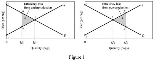
In figure -1 panel (a) and (b), the horizontal axis measures the quantity of bags and the vertical axis measures the
The inverse demand function can be derived as follows:
The inverse demand functions of
The inverse supply curve can be calculated as follows:
The inverse supply functions of
The inverse demand function and supply functions reveal that the producer willing price is $5 and the consumer willing price is $85. The equilibrium price is $45. The total surplus can be calculated as follows:
The total surplus is $800.
The consumer surplus can be calculated as follows:
The consumer surplus is $400.
Concept Introduction:
Consumer surplus: It refers to the variation in the probable charge of a product that the consumer intends to pay and the actual price that he has already paid.
Subpart (b):
The consumer surplus, total surplus and deadweight loss.
Subpart (b):
Explanation of Solution
The consumer willing price at Q2 level of output (15 units) can be calculated by substituting the Q2 level of output to the inverse demand function.
The consumer new willing price is $55.
The producer willing price at Q2 level of output (15 units) can be calculated by substituting the Q2 level of output into the inverse supply function.
The producer’s new willing price is $35.
The deadweight loss can be calculated as follows:
The deadweight loss is $50.
The total surplus can be calculated as follows:
The total surplus is $750.
Concept Introduction:
Consumer surplus: It refers to the variation in the probable charge of a product that the consumer intends to pay and the actual price that he has already paid.
Producer surplus: It refers to the variation in the probable price that the producer intends to sell and the actual price that he has already sold.
Subpart c):
The consumer surplus, total surplus and deadweight loss.
Subpart c):
Explanation of Solution
The consumer willing price at Q3 level of output (27 units) can be calculated by substituting the Q3 level of output to the inverse demand function.
The consumer new willing price is $31.
The producer willing price at Q3 level of output (127 units) can be calculated by substituting the Q3 level of output to the inverse supply function.
The producer new willing price is $59.
The deadweight loss can be calculated as follows:
The deadweight loss is $98.
The total surplus can be calculated as follows:
The total surplus is $702.
Concept Introduction:
Consumer surplus: It refers to the variation in the probable charge of a product that the consumer intends to pay and the actual price that he has already paid.
Producer surplus: It refers to the variation in the probable price that the producer intends to sell and the actual price that he has already sold.
Want to see more full solutions like this?
Chapter 4 Solutions
Macroeconomics: Principles, Problems, & Policies

- Discuss the impact of exchange rate volatility on the economy and its impact on your organisation. Make use of the relevant diagrams.arrow_forwardMacroeconomic policies have different effects on the price level and output (national income). Discuss the impact of a monetary policy that seeks to encourage economic growth.arrow_forwardCan you please help with this one. Some economists argue that taxing consumption is more efficient than taxing income. Following the same argument, the minister of finance of a country introduced a new tax for sugar based products “sugar tax” to promote healthy eating in the economy. Please use relevant diagrams to explain the impact of the tax on consumers, producers and the tax revenue when sugar is elastic and inelastic.arrow_forward
- profit maximizing and loss minamization fire dragon co mindtaparrow_forwardProblem 3 You are given the following demand for European luxury automobiles: Q=1,000 P-0.5.2/1.6 where P-Price of European luxury cars PA = Price of American luxury cars P, Price of Japanese luxury cars I= Annual income of car buyers Assume that each of the coefficients is statistically significant (i.e., that they passed the t-test). On the basis of the information given, answer the following questions 1. Comment on the degree of substitutability between European and American luxury cars and between European and Japanese luxury cars. Explain some possible reasons for the results in the equation. 2. Comment on the coefficient for the income variable. Is this result what you would expect? Explain. 3. Comment on the coefficient of the European car price variable. Is that what you would expect? Explain.arrow_forwardProblem 2: A manufacturer of computer workstations gathered average monthly sales figures from its 56 branch offices and dealerships across the country and estimated the following demand for its product: Q=+15,000-2.80P+150A+0.3P+0.35Pm+0.2Pc (5,234) (1.29) (175) (0.12) (0.17) (0.13) R²=0.68 SER 786 F=21.25 The variables and their assumed values are P = Price of basic model = 7,000 Q==Quantity A = Advertising expenditures (in thousands) = 52 P = Average price of a personal computer = 4,000 P. Average price of a minicomputer = 15,000 Pe Average price of a leading competitor's workstation = 8,000 1. Compute the elasticities for each variable. On this basis, discuss the relative impact that each variable has on the demand. What implications do these results have for the firm's marketing and pricing policies? 2. Conduct a t-test for the statistical significance of each variable. In each case, state whether a one-tail or two-tail test is required. What difference, if any, does it make to…arrow_forward
- You are the manager of a large automobile dealership who wants to learn more about the effective- ness of various discounts offered to customers over the past 14 months. Following are the average negotiated prices for each month and the quantities sold of a basic model (adjusted for various options) over this period of time. 1. Graph this information on a scatter plot. Estimate the demand equation. What do the regression results indicate about the desirability of discounting the price? Explain. Month Price Quantity Jan. 12,500 15 Feb. 12,200 17 Mar. 11,900 16 Apr. 12,000 18 May 11,800 20 June 12,500 18 July 11,700 22 Aug. 12,100 15 Sept. 11,400 22 Oct. 11,400 25 Nov. 11,200 24 Dec. 11,000 30 Jan. 10,800 25 Feb. 10,000 28 2. What other factors besides price might be included in this equation? Do you foresee any difficulty in obtaining these additional data or incorporating them in the regression analysis?arrow_forwardsimple steps on how it should look like on excelarrow_forwardConsider options on a stock that does not pay dividends.The stock price is $100 per share, and the risk-free interest rate is 10%.Thestock moves randomly with u=1.25and d=1/u Use Excel to calculate the premium of a10-year call with a strike of $100.arrow_forward
 Managerial Economics: A Problem Solving ApproachEconomicsISBN:9781337106665Author:Luke M. Froeb, Brian T. McCann, Michael R. Ward, Mike ShorPublisher:Cengage Learning
 Economics (MindTap Course List)EconomicsISBN:9781337617383Author:Roger A. ArnoldPublisher:Cengage Learning


