Subpart (a):
The consumer surplus , total surplus and deadweight loss .
Subpart (a):
Explanation of Solution
Figure -1 illustrates the
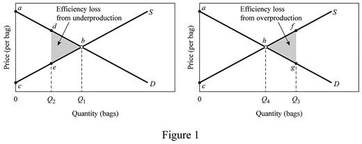
In figure -1 panel (a) and (b), the horizontal axis measures the quantity of bags and the vertical axis measures the
The inverse demand function can be derived as follows:
The inverse demand functions of
The inverse supply curve can be calculated as follows:
The inverse supply functions of
The inverse demand function and supply functions reveal that the producer willing price is $5 and the consumer willing price is $85. The equilibrium price is $45. The total surplus can be calculated as follows:
The total surplus is $800.
The consumer surplus can be calculated as follows:
The consumer surplus is $400.
Concept Introduction:
Consumer surplus: It refers to the variation in the probable charge of a product that the consumer intends to pay and the actual price that he has already paid.
Subpart (b):
The consumer surplus, total surplus and deadweight loss.
Subpart (b):
Explanation of Solution
The consumer willing price at Q2 level of output (15 units) can be calculated by substituting the Q2 level of output to the inverse demand function.
The consumer new willing price is $55.
The producer willing price at Q2 level of output (15 units) can be calculated by substituting the Q2 level of output into the inverse supply function.
The producer’s new willing price is $35.
The deadweight loss can be calculated as follows:
The deadweight loss is $50.
The total surplus can be calculated as follows:
The total surplus is $750.
Concept Introduction:
Consumer surplus: It refers to the variation in the probable charge of a product that the consumer intends to pay and the actual price that he has already paid.
Producer surplus: It refers to the variation in the probable price that the producer intends to sell and the actual price that he has already sold.
Subpart c):
The consumer surplus, total surplus and deadweight loss.
Subpart c):
Explanation of Solution
The consumer willing price at Q3 level of output (27 units) can be calculated by substituting the Q3 level of output to the inverse demand function.
The consumer new willing price is $31.
The producer willing price at Q3 level of output (127 units) can be calculated by substituting the Q3 level of output to the inverse supply function.
The producer new willing price is $59.
The deadweight loss can be calculated as follows:
The deadweight loss is $98.
The total surplus can be calculated as follows:
The total surplus is $702.
Concept Introduction:
Consumer surplus: It refers to the variation in the probable charge of a product that the consumer intends to pay and the actual price that he has already paid.
Producer surplus: It refers to the variation in the probable price that the producer intends to sell and the actual price that he has already sold.
Want to see more full solutions like this?
Chapter 4 Solutions
Economics: Principles, Problems, & Policies (McGraw-Hill Series in Economics) - Standalone book

- 1. Suppose that the two nations face the following benefits of pollution, B, and costs of abatement, C: BN = 10, Bs = 7; CN = 5, Cs = 4. Further assume that if the nation chooses to abate pollution, it still receives the benefits of pollution but now must pay the cost of abatement as well. a. Identify the payoffs that accrue to each nation under the four different possible outcomes of the game and present these payoffs in the normal form of the game. b. Recall that the term dominant strategy defines the condition that a player in a game would prefer to play that strategy (in this case either pollute or abate) regardless of the strategy chosen by the other player in the game. Does either nation have a dominant strategy in this game? If so, what is it? c. Identify the Nash equilibria, or non-cooperative equilibria, of this game.arrow_forwardagrody calming Inted 001 and me 2. A homeowner is concerned about the various air pollutants (e.g., benzene and methane) released in her house when she cooks with natural gas. She is considering replacing her gas oven and stove with an electric stove comprising an induction cooktop and convection oven. The new appliance costs $900 to purchase and install. Capping the old gas line costs an additional $150 (a one-time fee). The old line must be inspected for leaks each year after capping, at a cost of $35 for each inspection. a. If the homeowner plans to remain in the house for four more years and the discount rate is 4%, what is the minimum present value of the benefits that the homeowner would need to experience for this purchase to be justified based on its private net sub present value? b. While trying to understand how she might express the value of reduced exposure to indoor air pollutants in dollar terms, the homeowner consulted the EPA website and found estimates provided by…arrow_forwardAfter the ban is imposed, Joe’s firm switches to the more expensive biodegradable disposable cups. This increases the cost associated with each cup of coffee it produces. Which cost curve(s) will be impacted by the use of the more expensive biodegradable disposable cups? Why? Which cost curve(s) will not shift, and why not? Please use the table below to answer this question. For the second column (“Impacted? If so, how?”), please use one of the following three choices: No shift; Shifts up (i.e., increases: at nearly any given quantity, the cost goes up); or Shifts down (i.e., decreases: at nearly any given quantity, the cost goes down). $ Cost Curve Impacted? If so, how? Explanation of the Shift: Why or Why Not AFC No shift. Fix costs stay the same, regardless of quantity. Fixed cost is calculated as Fixed Cost/Quantity. Since fixed costs remain unchanged, AFC stays the same for each quantity. MC Shifts up. Since the biodegradable cups are more expensive, the…arrow_forward
- Styrofoam is non-biodegradable and is not easily recyclable. Many cities and at least one state have enacted laws that ban the use of polystyrene containers. These locales understand that banning these containers will force many businesses to turn to other more expensive forms of packaging and cups, but argue the ban is environmentally important. Shane owns a firm with a conventional production function resulting in U-shaped ATC, AVC, and MC curves. Shane's business sells takeout food and drinks that are currently packaged in styrofoam containers and cups. Graph the short-run AFC0, AVC0, ATC0, and MC0 curves for Shane's firm before the ban on using styrofoam containers.arrow_forwardd-farrow_forwarda-c pleasearrow_forward
- d-farrow_forwardPART II: Multipart Problems wood or solem of triflussd aidi 1. Assume that a society has a polluting industry comprising two firms, where the industry-level marginal abatement cost curve is given by: MAC = 24 - ()E and the marginal damage function is given by: MDF = 2E. What is the efficient level of emissions? b. What constant per-unit emissions tax could achieve the efficient emissions level? points) c. What is the net benefit to society of moving from the unregulated emissions level to the efficient level? In response to industry complaints about the costs of the tax, a cap-and-trade program is proposed. The marginal abatement cost curves for the two firms are given by: MAC=24-E and MAC2 = 24-2E2. d. How could a cap-and-trade program that achieves the same level of emissions as the tax be designed to reduce the costs of regulation to the two firms?arrow_forwardOnly #4 please, Use a graph please if needed to help provearrow_forward
- a-carrow_forwardFor these questions, you must state "true," "false," or "uncertain" and argue your case (roughly 3 to 5 sentences). When appropriate, the use of graphs will make for stronger answers. Credit will depend entirely on the quality of your explanation. 1. If the industry facing regulation for its pollutant emissions has a lot of political capital, direct regulatory intervention will be more viable than an emissions tax to address this market failure. 2. A stated-preference method will provide a measure of the value of Komodo dragons that is more accurate than the value estimated through application of the travel cost model to visitation data for Komodo National Park in Indonesia. 3. A correlation between community demographics and the present location of polluting facilities is sufficient to claim a violation of distributive justice. olsvrc Q 4. When the damages from pollution are uncertain, a price-based mechanism is best equipped to manage the costs of the regulator's imperfect…arrow_forwardFor environmental economics, question number 2 only please-- thank you!arrow_forward


 Microeconomics: Principles & PolicyEconomicsISBN:9781337794992Author:William J. Baumol, Alan S. Blinder, John L. SolowPublisher:Cengage Learning