
Subpart (a):
The consumer surplus , total surplus and deadweight loss .
Subpart (a):
Explanation of Solution
Figure -1 illustrates the
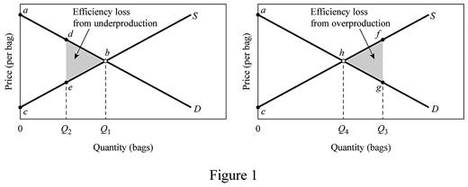
In figure -1 panel (a) and (b), the horizontal axis measures the quantity of bags and the vertical axis measures the
The inverse demand function can be derived as follows:
The inverse demand functions of
The inverse supply curve can be calculated as follows:
The inverse supply functions of
The inverse demand function and supply functions reveal that the producer willing price is $5 and the consumer willing price is $85. The equilibrium price is $45. The total surplus can be calculated as follows:
The total surplus is $800.
The consumer surplus can be calculated as follows:
The consumer surplus is $400.
Concept Introduction:
Consumer surplus: It refers to the variation in the probable charge of a product that the consumer intends to pay and the actual price that he has already paid.
Subpart (b):
The consumer surplus, total surplus and deadweight loss.
Subpart (b):
Explanation of Solution
The consumer willing price at Q2 level of output (15 units) can be calculated by substituting the Q2 level of output to the inverse demand function.
The consumer new willing price is $55.
The producer willing price at Q2 level of output (15 units) can be calculated by substituting the Q2 level of output into the inverse supply function.
The producer’s new willing price is $35.
The deadweight loss can be calculated as follows:
The deadweight loss is $50.
The total surplus can be calculated as follows:
The total surplus is $750.
Concept Introduction:
Consumer surplus: It refers to the variation in the probable charge of a product that the consumer intends to pay and the actual price that he has already paid.
Producer surplus: It refers to the variation in the probable price that the producer intends to sell and the actual price that he has already sold.
Subpart c):
The consumer surplus, total surplus and deadweight loss.
Subpart c):
Explanation of Solution
The consumer willing price at Q3 level of output (27 units) can be calculated by substituting the Q3 level of output to the inverse demand function.
The consumer new willing price is $31.
The producer willing price at Q3 level of output (127 units) can be calculated by substituting the Q3 level of output to the inverse supply function.
The producer new willing price is $59.
The deadweight loss can be calculated as follows:
The deadweight loss is $98.
The total surplus can be calculated as follows:
The total surplus is $702.
Concept Introduction:
Consumer surplus: It refers to the variation in the probable charge of a product that the consumer intends to pay and the actual price that he has already paid.
Producer surplus: It refers to the variation in the probable price that the producer intends to sell and the actual price that he has already sold.
Want to see more full solutions like this?
Chapter 4 Solutions
Economics (Irwin Economics)

- < Files 9:10 Fri Mar 21 Chapter+11-Public+Goods+and+Common+Res... The Economic Catch-22 By Robert J. Samuelson We are now in the "blame phase" of the economic cycle. As the housing slump deepens and financial markets swing erratically, we've embarked on the usual search for culprits. Who got us into this mess? Our investigations will doubtlessly reveal, as they already have, much wishful thinking and miscalculation. They will also find incompetence, predatory behavior and probably some criminality. But let me suggest that, though inevitable and necessary, this exercise is also simplistic and deceptive. -- business It assumes that, absent mistakes and misdeeds, we might remain in a permanent paradise of powerful income and wealth growth. The reality, I think, is that the economy follows its own Catch-22: By taking prosperity for granted, people perversely subvert prosperity. The more we managers, investors, consumers - think that economic growth is guaranteed and that risk and…arrow_forward2.) Using the line drawing tool, plot and label the isocost line. Carefully follow the instructions above, and only draw the required objects. FILL IN BLANK d. Now suppose the price of labour rises to $5 per unit, but the firm still wants to produce 500 tires per day. Explain how a cost-minimizing firm adjusts to this change (with no change in technology). A cost-minimizing firm will be producing on ▼ The samedifferently slopedparallel isocost line. The firm will use ▼ moresameless labour and ▼ less the same amount of more capital and produce on ▼ a higher point on the same a lower point on the same a lower a higher isoquant curve.arrow_forwardQK Using the graph on the right, determine how the firm should change the quantity of the production factors in order to reduce the costs. The firm that is producing at point A can reduce its costs for producing 2000 units by employing A. same capital and more labour. B. less capital and more labour. ○ C. less capital and the same labour. D. more capital and more labour. OE. more capital and less labour. C A B Q =4000 Q = 2000 C Isocost line QLarrow_forward
- PL Suppose the price ratio is the same along isocost PK lines A and B. In the figure at right, the difference between isocost line A and isocost line B is that A. the total cost is larger along B. B. the total cost is larger along A. OC. labour is relatively more expensive along A. ○ D. the level of output is lower along A. OE. both capital and labour are relatively cheaper along A. Capital B Labourarrow_forwardUsing the graph on the right, determine the per unit prices of capital and labour. 20- Given the information provided about the isocost lines, we know that the per unit price of capital is TC=$100 and the per unit price of labour is 16- TC $80 ○ A. $50; $20 ○ B. $2; $5 ○ C. $5; $2 ○ D. $20; $50 E. not determinable; not determinable Quantity of K 12 TC $60 TC $40 0 10 20 30 Quantity of L 40arrow_forwardThe diagram to the right contains isocost lines A and B. If the price of capital is the same for both lines, then the difference between isocost line A and isocost line B is that OA. the total cost is larger along B. B. the level of output is lower along A. C. both capital and labour are cheaper along A. OD. labour is more expensive along A. ○ E. labour is more expensive along B. Capital Labourarrow_forward
- For the firm whose cost curves are shown at right, the minimum efficient scale is ○ A. between 60 and 140 units of production. OB. about 20 units of production. OC. about 60 units of production. OD. about 100 units of production. OE. the level of fixed cost corresponding to SRATC2. SRATC₁ LRAC SRATC4 SRATC₂ SRATC3 เนด เad iso C 20 20 40 60 80 100 120 140 160 180 200 Output per Periodarrow_forwardSRATC₂ SRATC3 In the figure, increasing long-run average total costs for the firm are confined to the output range OA. where the LRAC curve is downward sloping. B. above 80 units of output. O C. above 50 units of output. OD. between 50 and 80 units of output. SRATC₁ OE. between 10 and 100 units of output. ---- SRATC LRAC 10 20 30 40 50 60 70 80 90 100 Output per Periodarrow_forwardFor the firm whose cost curves are shown at right, the minimum efficient scale is OA. between 10 and 50 units of production. OB. about 80 units of production. O C. the level of fixed cost corresponding to SRATC₁. OD. about 10 units of production. ○ E. about 50 units of production. Cost per Unit SRATC₁ LRAC SRATC2 SRATC4 SRATC3 10 20 30 40 50 60 70 80 Output per Period 90 100arrow_forward
- • 3 different people working at any companies under the BPO industry in the Philippines. • What are the 3 different Vision, Mission, Duties and Responsibilities and Career Path of these people in their companies under the BPO industry?arrow_forwardModule 6 ⚫(1902) Buckner C X | (1902) How to d x (1902) Buckner F X (1902) Productic X WP Videoplayer Canvas Login | Ir x | + Σ R mybrcc.instructure.com/courses/417310/discussion_topics/3420114?module_item_id=20155705 Spring 2025 Home Announcements Modules Syllabus Grades 8 People BRCC-_Library DLASC Module 6 Discussion - Business Costs Relaunch to update For this discussion, think about where you work or a business you have a significant amount of knowledge about. What is a common product that the business sells? What are the main costs the business has to incur in order to be able to sell that product? Which of these costs are fixed and which are variable? How much additional costs would be incurred if it were to sell one additional unit of that product (marginal cost)? Write a discussion thread about this business, the product it commonly sells, and your answers to the above questions. Also, respond to at least two threads created by your classmates. In these responses, share what…arrow_forwardRefer to the video to answer the following: • what are all the key policies or all the strategies the Philippine government should prioritize to accelerate sustainable economic growth? • these should consider the Philippines current economic challenges, including inflation, unemployment, and the need for digital transformation. "The Philippines' Strong Economic Growth" (YouTube link: https://youtu.be/1YtEoGp2ZeM?siJQfIv5kbu0txVsLL.)arrow_forward


 Microeconomics: Principles & PolicyEconomicsISBN:9781337794992Author:William J. Baumol, Alan S. Blinder, John L. SolowPublisher:Cengage Learning