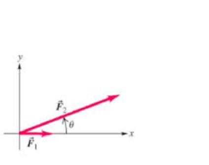
As shown in Figure 4.40, force vector F → 1 always points in the + x direction, but F → 2 makes an angle θ with the + x axis. A physics student is given the task of graphically determining the x and y components of the sum of these vectors, F → = F 1 → + F 2 → , for several different values of θ . The magnitudes of F 1 → and F 2 → remain unchanged; only the angle θ is varied. The table shows the student’s results: Figure 4.40 Problem 43. θ F x (N) F y (N) 20* 11.4 3.1 35* 10.4 5.2 60* 7.5 7.8 75* 5.3 8.7 (a) Write an expression for F in terms of θ F 1 and F 2 . (b) Make a linearized graph of the x component data with the value F , values on the y axis and the appropriate trig function of 0 on the x axis. (c) Draw a best-fit line through your plotted points and use this line to determine the magnitude F 1 and F 2 . (d) Repeat this process for the F 1 data and compare your result with what you obtained in part(c).
As shown in Figure 4.40, force vector F → 1 always points in the + x direction, but F → 2 makes an angle θ with the + x axis. A physics student is given the task of graphically determining the x and y components of the sum of these vectors, F → = F 1 → + F 2 → , for several different values of θ . The magnitudes of F 1 → and F 2 → remain unchanged; only the angle θ is varied. The table shows the student’s results: Figure 4.40 Problem 43. θ F x (N) F y (N) 20* 11.4 3.1 35* 10.4 5.2 60* 7.5 7.8 75* 5.3 8.7 (a) Write an expression for F in terms of θ F 1 and F 2 . (b) Make a linearized graph of the x component data with the value F , values on the y axis and the appropriate trig function of 0 on the x axis. (c) Draw a best-fit line through your plotted points and use this line to determine the magnitude F 1 and F 2 . (d) Repeat this process for the F 1 data and compare your result with what you obtained in part(c).
As shown in Figure 4.40, force vector
F
→
1
always points in the +x direction, but
F
→
2
makes an angle θ with the +x axis. A physics student is given the task of graphically determining the x and y components of the sum of these vectors,
F
→
=
F
1
→
+
F
2
→
, for several different values of θ. The magnitudes of
F
1
→
and
F
2
→
remain unchanged; only the angle θ is varied. The table shows the student’s results:
Figure 4.40
Problem 43.
θ
Fx(N)
Fy(N)
20*
11.4
3.1
35*
10.4
5.2
60*
7.5
7.8
75*
5.3
8.7
(a) Write an expression for F in terms of θ F1 and F2. (b) Make a linearized graph of the x component data with the value F, values on the y axis and the appropriate trig function of 0 on the x axis. (c) Draw a best-fit line through your plotted points and use this line to determine the magnitude F1 and F2. (d) Repeat this process for the F1 data and compare your result with what you obtained in part(c).
The cylindrical beam of a 12.7-mW laser is 0.920 cm in diameter. What is the rms value of the electric field?
V/m
Consider a rubber rod that has been rubbed with fur to give the rod a net negative charge, and a glass rod that has been rubbed with silk to give it a net positive charge. After being charged by contact by the fur and silk...?
a. Both rods have less mass
b. the rubber rod has more mass and the glass rod has less mass
c. both rods have more mass
d. the masses of both rods are unchanged
e. the rubber rod has less mass and the glass rod has mroe mass
8) 9)
Chapter 4 Solutions
Masteringphysics With Pearson Etext - Valuepack Access Card - For College Physics
Campbell Essential Biology with Physiology (5th Edition)
Knowledge Booster
Learn more about
Need a deep-dive on the concept behind this application? Look no further. Learn more about this topic, physics and related others by exploring similar questions and additional content below.


 Principles of Physics: A Calculus-Based TextPhysicsISBN:9781133104261Author:Raymond A. Serway, John W. JewettPublisher:Cengage Learning
 Classical Dynamics of Particles and SystemsPhysicsISBN:9780534408961Author:Stephen T. Thornton, Jerry B. MarionPublisher:Cengage Learning
 University Physics Volume 1PhysicsISBN:9781938168277Author:William Moebs, Samuel J. Ling, Jeff SannyPublisher:OpenStax - Rice University
 College PhysicsPhysicsISBN:9781305952300Author:Raymond A. Serway, Chris VuillePublisher:Cengage Learning
 Physics for Scientists and Engineers: Foundations...PhysicsISBN:9781133939146Author:Katz, Debora M.Publisher:Cengage Learning
 College PhysicsPhysicsISBN:9781285737027Author:Raymond A. Serway, Chris VuillePublisher:Cengage Learning