Concept explainers
Videos
a.
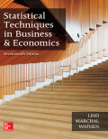
Construct box plot of the variable price.
Identify whether there are outliers or not.
Find the
Find the first
Find the third quartile value.
a.
Answer to Problem 37CE
Output of box plot for the variable price using MINITAB software is,
Yes, there are 3 outliers in the dataset.
The median price is 3,733.
The first quartile value is 1,478.
The third quartile value is 6,141.
Explanation of Solution
Calculation:
Step by step procedure to obtain boxplot using MINITAB software is given as,
- Choose Graph > Boxplot.
- In Graph variables enter the columns Price.
- Click OK.
Outliers:
In the boxplot, the outlier is represented using asterisk. In the boxplot of data set there are 3 asterisks representing outliers. Hence, there are three outliers in the dataset.
Median:
The median is the middle value of the data set. In the boxplot, the line in middle of the box represents median of the dataset. The line corresponds to value 3,733.
Hence, the median value is 3,733.
First quartile:
The border line towards the left side of the box represents the value of first quartile. In this box plot, the line of the box on left side corresponds to the value approximately 1,478.
Hence, the third quartile value is 6,141.
Third quartile:
The border line towards the right side of the box represents the value of third quartile. In this box plot, the line of the box on right side corresponds to the value approximately 6,141.
Hence, the first quartile value is 1,478.
b.
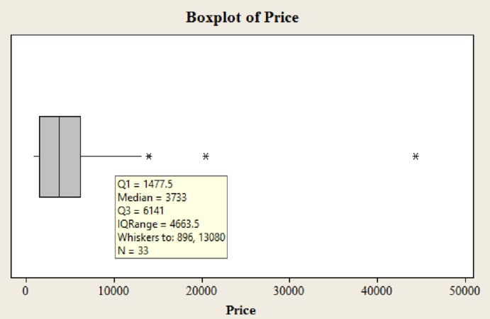
Construct box plot of the variable size.
Identify whether there are outliers or not.
Find the median price.
Find the first quartile value.
Find the third quartile value.
b.
Answer to Problem 37CE
Output of box plot for the variable size using MINITAB software is,
Yes, there are 3 outliers in the dataset.
The median price is 0.84.
The first quartile value is 0.515.
The third quartile value is 1.12.
Explanation of Solution
Calculation:
Step by step procedure to obtain boxplot using MINITAB software is given as,
- Choose Graph > Boxplot.
- In Graph variables enter the columns Size.
- Click OK.
Outliers:
In the boxplot, the outlier is represented using asterisk. In the boxplot of data set there are 3 asterisks representing outliers. Hence, there are three outliers in the dataset.
Median:
The median is the middle value of the data set. In the boxplot, the line in middle of the box represents median of the dataset. The line corresponds to value 0.84.
Hence, the median value is 0.84.
First quartile:
The border line towards the left side of the box represents the value of first quartile. In this box plot, the line of the box on left side corresponds to the value approximately 0.515.
Hence, the third quartile value is 0.515.
Third quartile:
The border line towards the right side of the box represents the value of third quartile. In this box plot, the line of the box on right side corresponds to the value approximately 1.12.
Hence, the first quartile value is 1.12.
c.
Construct
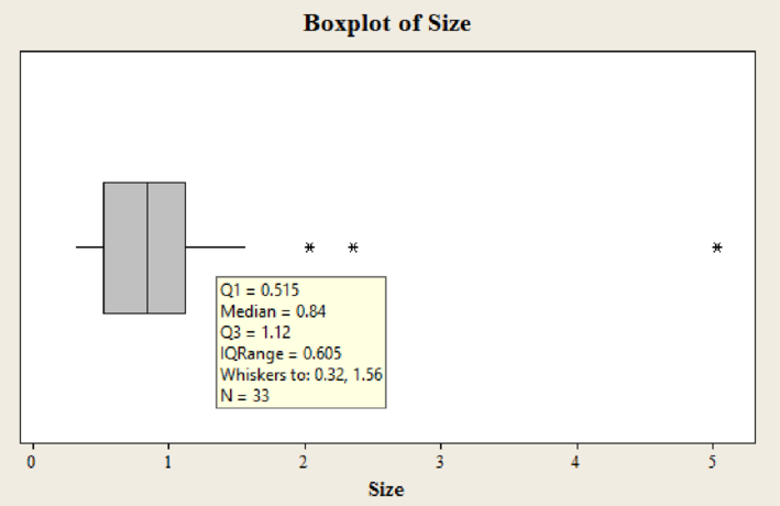
Identify whether there is association between the two variables or not.
Identify whether association is direct or indirect.
Identify whether any point seems to be different from the others.
c.
Answer to Problem 37CE
Output of scatter diagram for variables price and size using MINITAB software is,
Yes, there is association between the variables price and size.
The association is direct.
Yes, the first observation of both the price and size is large when compared to other observations.
Explanation of Solution
Calculation:
Step by step procedure to obtain scatter diagram using MINITAB software is given as,
- Choose Graph > Scatterplot > select Simple.
- In Y variable enter the column Price.
- In X variable enter the column Size.
- Click OK.
In the scatter diagram it can be observed that, the Price has increased as the Size increases indicating that the association between the variables.
Hence, there is association between the variables price and size
The relation is said to be direct if value of one variable increases due to effect of another variable. From the scatter diagram, the value of Price has increased as the Size increases indicating a direct or positive association.
Hence, the association is direct.
From the scatter diagram, it can be observed that one of the observations corresponding to the value of 5.03 carats for size and $44,312 for price is far from all the other observations. Hence, one point seems to be different from the others.
d.
Construct a
Find the most common cut grade.
Find the most common shape.
Find the most common combination of cut grade and shape.
d.
Answer to Problem 37CE
The contingency table for the variables shape and cut grade is,
| Shape | Cut Grade | |||||
| Average | Good | Ideal | Premium | Ultra Ideal | Total | |
| Emerald | 0 | 0 | 1 | 0 | 0 | 1 |
| Marquise | 0 | 2 | 0 | 1 | 0 | 3 |
| Oval | 0 | 0 | 0 | 1 | 0 | 1 |
| Princess | 1 | 0 | 2 | 2 | 0 | 5 |
| Round | 1 | 3 | 3 | 13 | 3 | 23 |
| Total | 2 | 5 | 6 | 17 | 3 | 33 |
The most common cut grade is premium.
The most common shape is round.
The most common combination of cut grade and shape is premium and round.
Explanation of Solution
Calculation:
Contingency table:
A table that is used for classifying observations based on the two identifiable characteristics is termed as contingency table. It is used for summarizing two variables.
The variable cut grade is classified into 5 different categories ‘average, good, ideal, premium, ultra ideal’. The variable shape is classified into 5 different categories ‘emerald, marquise, oval, princess, and round’.
Count the number of cut grades are average with shape of emerald. From the data, there is no combination of average cut grades with shape of emerald. Hence, the frequency is 0.
Similarly, count the frequency for each of the possible combination of cut grade and shape. Then calculate the totals for each column and row. The contingency table is obtained as below,
| Shape | Cut Grade | |||||
| Average | Good | Ideal | Premium | Ultra Ideal | Total | |
| Emerald | 0 | 0 | 1 | 0 | 0 | 1 |
| Marquise | 0 | 2 | 0 | 1 | 0 | 3 |
| Oval | 0 | 0 | 0 | 1 | 0 | 1 |
| Princess | 1 | 0 | 2 | 2 | 0 | 5 |
| Round | 1 | 3 | 3 | 13 | 3 | 23 |
| Total | 2 | 5 | 6 | 17 | 3 | 33 |
The cut grade ‘Premium’ has a total of 17, which is large when compared to other cut grades. This shows that, the most common cut grade of diamonds is ‘Premium.
Hence, the most common cut grade is premium.
The shape ‘Round’ has a total of 23, which is large when compared to other shapes. This shows that, the most common shape of diamonds is ‘Round’.
Hence, the most common shape is round.
The combination of cut grade ‘Premium’ and shape ‘Round’ has a total of 13, which is large when compared to other combinations. This shows that, the most common combination of diamonds is cut grade ‘Premium’ and shape ‘Round’.
Hence, the most common combination of cut grade and shape is premium and round.
Want to see more full solutions like this?
Chapter 4 Solutions
EBK STATISTICAL TECHNIQUES IN BUSINESS


- This is the information about the actors who won the Best Actor Oscar: Best actors 44 41 62 52 41 34 34 52 41 37 38 34 32 40 43 56 41 39 49 57 35 30 39 41 44 41 38 42 52 51 49 35 47 31 47 37 57 42 45 42 44 62 43 42 48 49 56 38 60 30 40 42 36 76 39 53 45 36 62 43 51 32 42 54 52 37 38 32 45 60 46 40 36 47 29 43 a. What is the variable? What type? b. Construct an interval-frequency table, with columns containing: class mark, absolute frequency, relative frequency, cumulative frequency, cumulative relative frequency, and percentage frequency.arrow_forwardans c plsarrow_forwardCritically analyze the following graph and, based on statistical information, indicate the type of error it presents IN NO MORE THAN 3 LINES SCOTCEN POLL OF POLLS SHOULD SCOTLAND BE INDEPENDENT? NO 52% YES 58% LIVE CAW NAS & 28.30 HAS KILLED MORE THAN 2,600 IN WEST AFRICA, WORLD HEALTH ORG. BROOKEBCNNarrow_forward
- Critically analyze the following graph and, based on statistical information, indicate the type of error it presents IN NO MORE THAN 3 LINES PRESIDENTIAL PREFERENCES RODOLFO CARTER 3% (+2pts) EVELYN MATTHEI 22% (+6pts) With the exception of President Boric, could you tell me who you would like to be the next president of Chile? CAMILA VALLEJO 4% (+2pts) JOSÉ ANTONIO KAST 19% (+5pts) MICHELLE BACHELET 6% (+1pts)arrow_forwardCritically analyze the following graph and, based on statistical information, indicate the type of error it presents IN NO MORE THAN 3 LINES 13% APPROVE 4% DOESN'T KNOW DOESN'T RESPOND 5% NEITHER APPROVES NOR DISAPPROVES 78% DISAPPROVES SURVEY PRESIDENTIAL APPROVAL DROPS TO 13%arrow_forwardPlease help with this following question I'm not too sure if question (a) and (b) are correct and not sure how to calculate (c) The csv data is below "","New","Current" "1","67",66 "2","77",73 "3","76",73 "4","76",76 "5","77",79 "6","84",76 "7","71",78 "8","84",72 "9","73",76 "10","71",73 "11","72",77 "12","70",72 "13","75",72 "14","84",71 "15","77",73 "16","65",72 "17","69",73 "18","71",73 "19","79",71 "20","75",78 "21","76",69 "22","73",74 "23","76",71 "24","64",74 "25","81",78 "26","79",76 "27","70",77 "28","79",71 "29","84",73 "30","79",69 "31","69",72 "32","81",76 "33","77",70 "34","77",71 "35","71",69 "36","67",72 "37","70",76 "38","77",73 "39","82",73 "40","72",73arrow_forward
- Please help me answer the following question(c) A previous study found that 15% of nurses reported participating in mental health support programs.From the 96% found in (b) , can you conclude that proportion of nurses reported participating in mental health support programs p(current), has changed from the previous study?(Yes/No) because the confidence interval in (b) (captures/does not capture) 15%.(d) Refer to your answer in (b) : The Alberta Nurses Association expects that not more than 23 % of nurses will participate in the survey on mental health support programs. Given the result in part (b) can we conclude that this expectation is reasonable?(Yes/No) because the (upper bound/lower bound) of the 96% confidence interval is (less than/not less than/greater than) 23%. The Alberta Nursing Association conducts an annual survey to estimate the proportion of nurses who participate in mental health support programs. The most recent application of this survey involved a random sample of…arrow_forwardPlease help me solve this questionThis is what was in the csv file:"","Diabetic","Heart Disease""1",32644,30646"2",789,1670"3",12802,36274"4",2177,5011"5",1910,3300"6",3320,4256"7",61425,39053"8",19768,28635"9",19502,39546"10",5642,12182"11",107864,152098"12",29918,60433"13",2397,3550"14",41559,34705"15",49169,57948"16",72853,83100"17",2155,2873"18",140220,134517"19",28181,26212"20",18850,38637"21",69564,68582"22",13897,12613"23",6868,9138"24",9735,4767"25",12102,13447"26",36571,50010"27",44665,55141"28",26620,33970"29",25525,29766"30",14167,20206Q(b) From this, the relationship between these two variables is (non-existent/positive/negative) . I can categorize this relationship as being (strong/weak/moderate).Q(c) Drop down is (+/-)Q(d) Drop downs in order are __% of the (average/median/variation/standard deviation) in the (the number of people diagnosed with heart disease/the number of people diagnosed with diabetes)−variable can be explained by its (linear relationship/relationship)…arrow_forwardPlease help me answer the following question The drop down for question (e, f, and g) is (YES/NO) Based on the P-value above, the assumption of equal variances among the four machines (Is Met/Is Not Met) Based on the data, the average fill for machine 3 is (statistically lower than/statistically higher than/the same as/not statistically different than/statistically different than/Hard to say then when comparing to/Refuse to say when comparing to) machine 1.arrow_forward
- Business Discussarrow_forward1 for all k, and set o (ii) Let X1, X2, that P(Xkb) = x > 0. Xn be independent random variables with mean 0, suppose = and Var Xk. Then, for 0x) ≤2 exp-tx+121 Στ k=1arrow_forwardLemma 1.1 Suppose that g is a non-negative, non-decreasing function such that E g(X) 0. Then, E g(|X|) P(|X|> x) ≤ g(x)arrow_forward
 Big Ideas Math A Bridge To Success Algebra 1: Stu...AlgebraISBN:9781680331141Author:HOUGHTON MIFFLIN HARCOURTPublisher:Houghton Mifflin Harcourt
 Glencoe Algebra 1, Student Edition, 9780079039897...AlgebraISBN:9780079039897Author:CarterPublisher:McGraw Hill
 Holt Mcdougal Larson Pre-algebra: Student Edition...AlgebraISBN:9780547587776Author:HOLT MCDOUGALPublisher:HOLT MCDOUGAL