
Concept explainers
Videos
a.
Find the mean of the number of members per component.
Find the
Find the standard deviation of the number of members per component.
a.
Answer to Problem 36CE
The mean of the number of members per component is 348.5.
The median of the number of members per component is 276.
The standard deviation of the number of members per component is 277.4.
Explanation of Solution
Calculation:
Step by step procedure to obtain mean, median and standard deviation using MINITAB software is given as,
- Choose Stat > Basic Statistics > Display
Descriptive Statistics . - In Variables enter the columns Membership.
- Choose option statistics, and select Mean, Median, Standard deviation.
- Click OK.
Output using MINITAB software is given below:
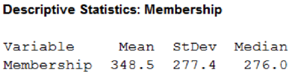
Hence, mean of the number of members per component is 348.5, the median is 276 and the standard deviation is 277.4.
b.
Find the coefficient of skewness.
Identify the shape of the distribution of component size.
b.
Answer to Problem 36CE
The coefficient of skewness is 1.17.
The shape of the distribution of component size is positive skewness.
Explanation of Solution
Calculation:
Step by step procedure to obtain skewness using MINITAB software is given as,
- Choose Stat > Basic Statistics > Graphical Summary.
- In Variables enter the columns Membership.
- Click OK.
Output using MINITAB software is given below:
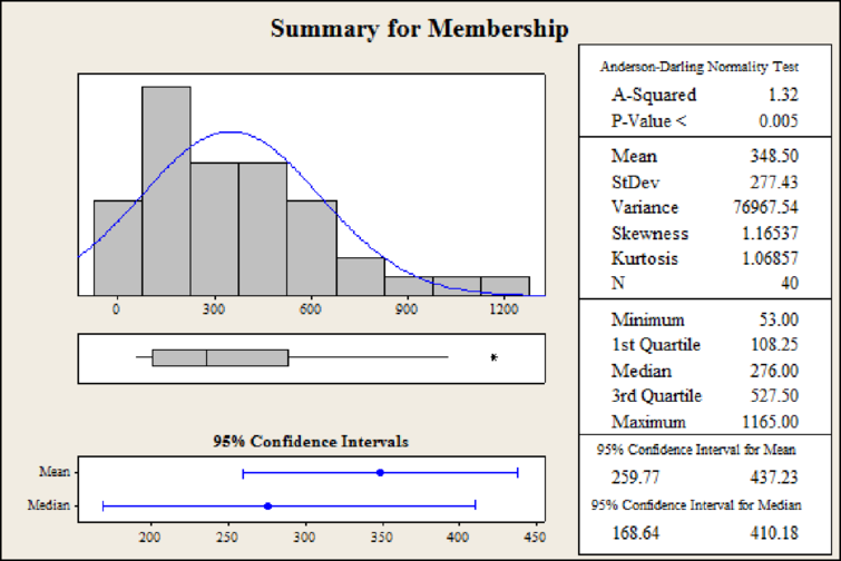
Hence, the value of coefficient of skewness is 1.17.
From the plot, it can be observed that most of the values are extended towards right indicating that distribution of component size is skewed to the right or positively skewed.
c.
Find the first
Find the third quartile.
c.
Answer to Problem 36CE
The first quartile is 108.25.
The third quartile is 527.50.
Explanation of Solution
Calculation:
Location of percentile:
The formula for percentile is,
In the formula, P denotes the location of the percentile and n denotes the total number of observations.
First quartile:
The first quartile represents the 25% of observation lies below first quartile. That is
Substitute,
The position of first quartile is 10.25th value in the dataset.
Hence, the first quartile is 108.25.
Third quartile:
The third quartile represents the 75% of observation lies above third quartile. That is
Substitute,
The position of third quartile is 30.75th value in the dataset.
Hence, the third quartile is 527.50.
d.
Construct a boxplot.
Identify whether there are outliers or not.
Find the components that are outliers.
Find the limits for outliers.
d.
Answer to Problem 36CE
The boxplot is,
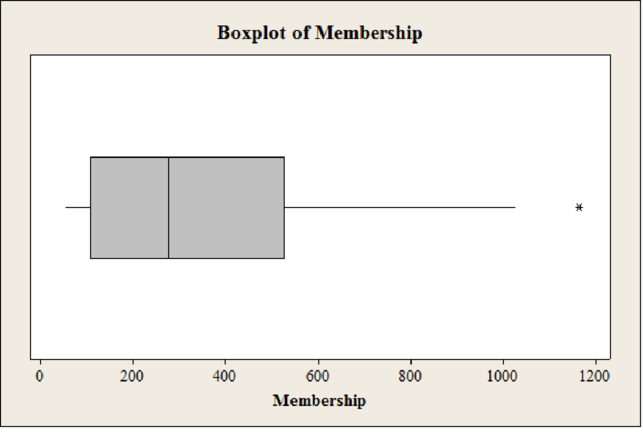
Yes, there are outliers.
The limits for outliers are (0; 1,156.375).
The component that is outlier is California.
Explanation of Solution
Calculation:
Step by step procedure to obtain boxplot using MINITAB software is given as,
- Choose Graph > Boxplot.
- In Graph variables enter the columns Membership.
- Click OK.
In the boxplot, the outlier is represented using asterisk. In the boxplot of data set there is one asterisk representing outliers. Hence, there is one outlier in the dataset.
Limits for detecting outliers:
Any data value beyond the below points are considered as outliers.
Substitute,
Since the membership cannot be negative, the lower point is considered as 0.
The points below 0 and above 1,156.375 are considered as outliers. Hence the limits for outliers are (0; 1,156.375).
The membership corresponding to state ‘California’ is 1,165, which is above the upper limit 1,156.375. This shows that, California is a component of outlier.
Hence, the component that is outlier is California.
Want to see more full solutions like this?
Chapter 4 Solutions
STATISTICAL TECHNIQUES-ACCESS ONLY


- Please could you check my answersarrow_forwardLet Y₁, Y2,, Yy be random variables from an Exponential distribution with unknown mean 0. Let Ô be the maximum likelihood estimates for 0. The probability density function of y; is given by P(Yi; 0) = 0, yi≥ 0. The maximum likelihood estimate is given as follows: Select one: = n Σ19 1 Σ19 n-1 Σ19: n² Σ1arrow_forwardPlease could you help me answer parts d and e. Thanksarrow_forward
- When fitting the model E[Y] = Bo+B1x1,i + B2x2; to a set of n = 25 observations, the following results were obtained using the general linear model notation: and 25 219 10232 551 XTX = 219 10232 3055 133899 133899 6725688, XTY 7361 337051 (XX)-- 0.1132 -0.0044 -0.00008 -0.0044 0.0027 -0.00004 -0.00008 -0.00004 0.00000129, Construct a multiple linear regression model Yin terms of the explanatory variables 1,i, x2,i- a) What is the value of the least squares estimate of the regression coefficient for 1,+? Give your answer correct to 3 decimal places. B1 b) Given that SSR = 5550, and SST=5784. Calculate the value of the MSg correct to 2 decimal places. c) What is the F statistics for this model correct to 2 decimal places?arrow_forwardCalculate the sample mean and sample variance for the following frequency distribution of heart rates for a sample of American adults. If necessary, round to one more decimal place than the largest number of decimal places given in the data. Heart Rates in Beats per Minute Class Frequency 51-58 5 59-66 8 67-74 9 75-82 7 83-90 8arrow_forwardcan someone solvearrow_forward
- QUAT6221wA1 Accessibility Mode Immersiv Q.1.2 Match the definition in column X with the correct term in column Y. Two marks will be awarded for each correct answer. (20) COLUMN X Q.1.2.1 COLUMN Y Condenses sample data into a few summary A. Statistics measures Q.1.2.2 The collection of all possible observations that exist for the random variable under study. B. Descriptive statistics Q.1.2.3 Describes a characteristic of a sample. C. Ordinal-scaled data Q.1.2.4 The actual values or outcomes are recorded on a random variable. D. Inferential statistics 0.1.2.5 Categorical data, where the categories have an implied ranking. E. Data Q.1.2.6 A set of mathematically based tools & techniques that transform raw data into F. Statistical modelling information to support effective decision- making. 45 Q Search 28 # 00 8 LO 1 f F10 Prise 11+arrow_forwardStudents - Term 1 - Def X W QUAT6221wA1.docx X C Chat - Learn with Chegg | Cheg X | + w:/r/sites/TertiaryStudents/_layouts/15/Doc.aspx?sourcedoc=%7B2759DFAB-EA5E-4526-9991-9087A973B894% QUAT6221wA1 Accessibility Mode பg Immer The following table indicates the unit prices (in Rands) and quantities of three consumer products to be held in a supermarket warehouse in Lenasia over the time period from April to July 2025. APRIL 2025 JULY 2025 PRODUCT Unit Price (po) Quantity (q0)) Unit Price (p₁) Quantity (q1) Mineral Water R23.70 403 R25.70 423 H&S Shampoo R77.00 922 R79.40 899 Toilet Paper R106.50 725 R104.70 730 The Independent Institute of Education (Pty) Ltd 2025 Q Search L W f Page 7 of 9arrow_forwardCOM WIth Chegg Cheg x + w:/r/sites/TertiaryStudents/_layouts/15/Doc.aspx?sourcedoc=%7B2759DFAB-EA5E-4526-9991-9087A973B894%. QUAT6221wA1 Accessibility Mode Immersi The following table indicates the unit prices (in Rands) and quantities of three meals sold every year by a small restaurant over the years 2023 and 2025. 2023 2025 MEAL Unit Price (po) Quantity (q0)) Unit Price (P₁) Quantity (q₁) Lasagne R125 1055 R145 1125 Pizza R110 2115 R130 2195 Pasta R95 1950 R120 2250 Q.2.1 Using 2023 as the base year, compute the individual price relatives in 2025 for (10) lasagne and pasta. Interpret each of your answers. 0.2.2 Using 2023 as the base year, compute the Laspeyres price index for all of the meals (8) for 2025. Interpret your answer. Q.2.3 Using 2023 as the base year, compute the Paasche price index for all of the meals (7) for 2025. Interpret your answer. Q Search L O W Larrow_forward
- QUAI6221wA1.docx X + int.com/:w:/r/sites/TertiaryStudents/_layouts/15/Doc.aspx?sourcedoc=%7B2759DFAB-EA5E-4526-9991-9087A973B894%7 26 QUAT6221wA1 Q.1.1.8 One advantage of primary data is that: (1) It is low quality (2) It is irrelevant to the purpose at hand (3) It is time-consuming to collect (4) None of the other options Accessibility Mode Immersive R Q.1.1.9 A sample of fifteen apples is selected from an orchard. We would refer to one of these apples as: (2) ھا (1) A parameter (2) A descriptive statistic (3) A statistical model A sampling unit Q.1.1.10 Categorical data, where the categories do not have implied ranking, is referred to as: (2) Search D (2) 1+ PrtSc Insert Delete F8 F10 F11 F12 Backspace 10 ENG USarrow_forwardepoint.com/:w:/r/sites/TertiaryStudents/_layouts/15/Doc.aspx?sourcedoc=%7B2759DFAB-EA5E-4526-9991-9087A 23;24; 25 R QUAT6221WA1 Accessibility Mode DE 2025 Q.1.1.4 Data obtained from outside an organisation is referred to as: (2) 45 (1) Outside data (2) External data (3) Primary data (4) Secondary data Q.1.1.5 Amongst other disadvantages, which type of data may not be problem-specific and/or may be out of date? W (2) E (1) Ordinal scaled data (2) Ratio scaled data (3) Quantitative, continuous data (4) None of the other options Search F8 F10 PrtSc Insert F11 F12 0 + /1 Backspaarrow_forward/r/sites/TertiaryStudents/_layouts/15/Doc.aspx?sourcedoc=%7B2759DFAB-EA5E-4526-9991-9087A973B894%7D&file=Qu Q.1.1.14 QUAT6221wA1 Accessibility Mode Immersive Reader You are the CFO of a company listed on the Johannesburg Stock Exchange. The annual financial statements published by your company would be viewed by yourself as: (1) External data (2) Internal data (3) Nominal data (4) Secondary data Q.1.1.15 Data relevancy refers to the fact that data selected for analysis must be: (2) Q Search (1) Checked for errors and outliers (2) Obtained online (3) Problem specific (4) Obtained using algorithms U E (2) 100% 高 W ENG A US F10 点 F11 社 F12 PrtSc 11 + Insert Delete Backspacearrow_forward
 Big Ideas Math A Bridge To Success Algebra 1: Stu...AlgebraISBN:9781680331141Author:HOUGHTON MIFFLIN HARCOURTPublisher:Houghton Mifflin Harcourt
 Glencoe Algebra 1, Student Edition, 9780079039897...AlgebraISBN:9780079039897Author:CarterPublisher:McGraw Hill
 Holt Mcdougal Larson Pre-algebra: Student Edition...AlgebraISBN:9780547587776Author:HOLT MCDOUGALPublisher:HOLT MCDOUGAL