
Concept explainers
(a)
The histogram frequency distribution, cumulative percentage distribution for each set of data and average speed.
Answer to Problem 10P
Explanation of Solution
Given:
Significance level of

Formula used:
Calculation:
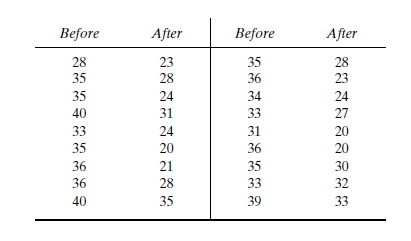
Before an increase in speed enforcement activities:
The speed ranges from 28 to 40 mi/h giving a speed range of 12. For five classes, the range per class is 2.4 mi/h. A frequency distribution table can then be prepared, as shown below in which the speed classes are listed in column 1 and the mid-values are in column 2. The number of observations for each class is listed in column 3 and the cumulative percentages of all observations are listed in column 6.
| 1 | 2 | 3 | 4 | 5 | 6 | 7 |
| Speed class (mi/h) | Class mid-value | Class frequency, | Percentage of class frequency | Cumulative percentage of class frequency | ||
| 28-30 | 29 | 4 | 116 | 13 | 13 | 139.24 |
| 31-33 | 32 | 5 | 160 | 17 | 30 | 42.05 |
| 34-36 | 35 | 12 | 420 | 40 | 70 | 0.12 |
| 37-39 | 38 | 6 | 228 | 20 | 90 | 57.66 |
| 40-42 | 41 | 3 | 123 | 10 | 100 | 111.63 |
| Total | 30 | 1047 | 350.7 |
Below Figure shows the frequency histogram for the data shown in above Table. The values in columns 2 and 3 of Table are used to draw the frequency histogram, where the abscissa represents the speeds and the ordinate the observed frequency in each class.

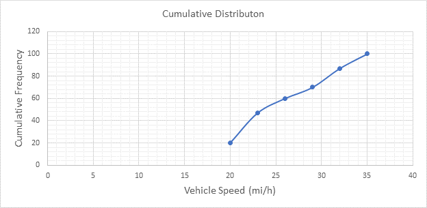
Below Figure shows the cumulative frequency distribution curve for the data given. In this case, the cumulative percentages in column 6 of above Table are plotted against the upper limit of each corresponding speed class. This curve gives the percentage of vehicles that are traveling at or below a given speed.

Determine the arithmetic mean speed:
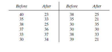
After an increase in speed enforcement activities:
The speed ranges from 20 to 37 mi/h giving a speed range of 17. For six classes, the range per class is 2.83 mi/h. A frequency distribution table can then be prepared, as shown below in which the speed classes are listed in column 1 and the mid-values are in column 2. The number of observations for each class is listed in column 3 and the cumulative percentages of all observations are listed in column 6.
| 1 | 2 | 3 | 4 | 5 | 6 | 7 |
| Speed class (mi/h) | Class mid-value | Class frequency, | Percentage of class frequency | Cumulative percentage of class frequency | ||
| 20-22 | 21 | 6 | 126 | 20 | 20 | 253.5 |
| 23-25 | 24 | 8 | 192 | 27 | 47 | 98 |
| 26-28 | 27 | 4 | 108 | 13 | 60 | 1 |
| 29-31 | 30 | 3 | 90 | 10 | 70 | 18.75 |
| 32-34 | 33 | 5 | 165 | 17 | 87 | 151.25 |
| 35-37 | 36 | 4 | 144 | 13 | 100 | 289 |
| Total | 30 | 825 | 811.5 |
Below Figure shows the frequency histogram for the data shown in above Table. The values in columns 2 and 3 of Table are used to draw the frequency histogram, where the abscissa represents the speeds and the ordinate the observed frequency in each class.

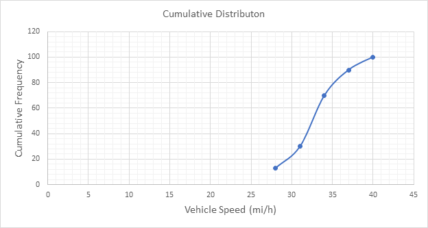
Below Figure shows the cumulative frequency distribution curve for the data given. In this case, the cumulative percentages in column 6 of above Table are plotted against the upper limit of each corresponding speed class. This curve gives the percentage of vehicles that are traveling at or below a given speed.

Determine the arithmetic mean speed:
Conclusion:
The average speeds of each set of data are 34.9 and 27.5 mi/h respectively.
(b)
The histogram frequency distribution, cumulative percentage distribution for each set of data and 85th percentile speed.
Answer to Problem 10P
Explanation of Solution
Given:
Significance level of

Calculation:
Before an increase in speed enforcement activities:
The speed ranges from 28 to 40 mi/h giving a speed range of 12. For five classes, the range per class is 2.4 mi/h. A frequency distribution table can then be prepared, as shown below in which the speed classes are listed in column 1 and the mid-values are in column 2. The number of observations for each class is listed in column 3 and the cumulative percentages of all observations are listed in column 6.
| 1 | 2 | 3 | 4 | 5 | 6 | 7 |
| Speed class (mi/h) | Class mid-value | Class frequency, | Percentage of class frequency | Cumulative percentage of class frequency | ||
| 28-30 | 29 | 4 | 116 | 13 | 13 | 139.24 |
| 31-33 | 32 | 5 | 160 | 17 | 30 | 42.05 |
| 34-36 | 35 | 12 | 420 | 40 | 70 | 0.12 |
| 37-39 | 38 | 6 | 228 | 20 | 90 | 57.66 |
| 40-42 | 41 | 3 | 123 | 10 | 100 | 111.63 |
| Total | 30 | 1047 | 350.7 |
Below Figure shows the frequency histogram for the data shown in above Table. The values in columns 2 and 3 of Table are used to draw the frequency histogram, where the abscissa represents the speeds and the ordinate the observed frequency in each class.

Below Figure shows the cumulative frequency distribution curve for the data given. In this case, the cumulative percentages in column 6 of above Table are plotted against the upper limit of each corresponding speed class. This curve gives the percentage of vehicles that are traveling at or below a given speed.

The 85th-percentile speed is obtained from the cumulative frequency distribution curve as 36 mi/h.
After an increase in speed enforcement activities:
The speed ranges from 20 to 37 mi/h giving a speed range of 17. For six classes, the range per class is 2.83 mi/h. A frequency distribution table can then be prepared, as shown below in which the speed classes are listed in column 1 and the mid-values are in column 2. The number of observations for each class is listed in column 3 and the cumulative percentages of all observations are listed in column 6.
| 1 | 2 | 3 | 4 | 5 | 6 | 7 |
| Speed class (mi/h) | Class mid-value | Class frequency, | Percentage of class frequency | Cumulative percentage of class frequency | ||
| 20-22 | 21 | 6 | 126 | 20 | 20 | 253.5 |
| 23-25 | 24 | 8 | 192 | 27 | 47 | 98 |
| 26-28 | 27 | 4 | 108 | 13 | 60 | 1 |
| 29-31 | 30 | 3 | 90 | 10 | 70 | 18.75 |
| 32-34 | 33 | 5 | 165 | 17 | 87 | 151.25 |
| 35-37 | 36 | 4 | 144 | 13 | 100 | 289 |
| Total | 30 | 825 | 811.5 |
Below Figure shows the frequency histogram for the data shown in above Table. The values in columns 2 and 3 of Table are used to draw the frequency histogram, where the abscissa represents the speeds and the ordinate the observed frequency in each class.

Below Figure shows the cumulative frequency distribution curve for the data given. In this case, the cumulative percentages in column 6 of above Table are plotted against the upper limit of each corresponding speed class. This curve gives the percentage of vehicles that are traveling at or below a given speed.

The 85th-percentile speed is obtained from the cumulative frequency distribution curve as 31.5 mi/h.
Conclusion:
The 85th-percentile speed for each set of data are 36 and 31.5 mi/h respectively.
(c)
The histogram frequency distribution, cumulative percentage distribution for each set of data and 15th percentile speed.
Answer to Problem 10P
Explanation of Solution
Given:
Significance level of


Calculation:
Before an increase in speed enforcement activities:
The speed ranges from 28 to 40 mi/h giving a speed range of 12. For five classes, the range per class is 2.4 mi/h. A frequency distribution table can then be prepared, as shown below in which the speed classes are listed in column 1 and the mid-values are in column 2. The number of observations for each class is listed in column 3 and the cumulative percentages of all observations are listed in column 6.
| 1 | 2 | 3 | 4 | 5 | 6 | 7 |
| Speed class (mi/h) | Class mid-value | Class frequency, | Percentage of class frequency | Cumulative percentage of class frequency | ||
| 28-30 | 29 | 4 | 116 | 13 | 13 | 139.24 |
| 31-33 | 32 | 5 | 160 | 17 | 30 | 42.05 |
| 34-36 | 35 | 12 | 420 | 40 | 70 | 0.12 |
| 37-39 | 38 | 6 | 228 | 20 | 90 | 57.66 |
| 40-42 | 41 | 3 | 123 | 10 | 100 | 111.63 |
| Total | 30 | 1047 | 350.7 |
Below Figure shows the frequency histogram for the data shown in above Table. The values in columns 2 and 3 of Table are used to draw the frequency histogram, where the abscissa represents the speeds and the ordinate the observed frequency in each class.
Below Figure shows the cumulative frequency distribution curve for the data given. In this case, the cumulative percentages in column 6 of above Table are plotted against the upper limit of each corresponding speed class. This curve gives the percentage of vehicles that are traveling at or below a given speed.

The 15th-percentile speed is obtained from the cumulative frequency distribution curve as 28.5 mi/h.
After an increase in speed enforcement activities:
The speed ranges from 20 to 37 mi/h giving a speed range of 17. For six classes, the range per class is 2.83 mi/h. A frequency distribution table can then be prepared, as shown below in which the speed classes are listed in column 1 and the mid-values are in column 2. The number of observations for each class is listed in column 3 and the cumulative percentages of all observations are listed in column 6.
| 1 | 2 | 3 | 4 | 5 | 6 | 7 |
| Speed class (mi/h) | Class mid-value | Class frequency, | Percentage of class frequency | Cumulative percentage of class frequency | ||
| 20-22 | 21 | 6 | 126 | 20 | 20 | 253.5 |
| 23-25 | 24 | 8 | 192 | 27 | 47 | 98 |
| 26-28 | 27 | 4 | 108 | 13 | 60 | 1 |
| 29-31 | 30 | 3 | 90 | 10 | 70 | 18.75 |
| 32-34 | 33 | 5 | 165 | 17 | 87 | 151.25 |
| 35-37 | 36 | 4 | 144 | 13 | 100 | 289 |
| Total | 30 | 825 | 811.5 |
Below Figure shows the frequency histogram for the data shown in above Table. The values in columns 2 and 3 of Table are used to draw the frequency histogram, where the abscissa represents the speeds and the ordinate the observed frequency in each class.
Below Figure shows the cumulative frequency distribution curve for the data given. In this case, the cumulative percentages in column 6 of above Table are plotted against the upper limit of each corresponding speed class. This curve gives the percentage of vehicles that are traveling at or below a given speed.
The 15th-percentile speed is obtained from the cumulative frequency distribution curve as 0 mi/h.
Conclusion:
The 15th-percentile speed for each set of data are 28.5 and 0 mi/h respectively.
(d)
The histogram frequency distribution, cumulative percentage distribution for each set of data and mode.
Answer to Problem 10P
35 mi/h and 24 mi/h
Explanation of Solution
Given:
Significance level of


Calculation:
Before an increase in speed enforcement activities:
The speed ranges from 28 to 40 mi/h giving a speed range of 12. For five classes, the range per class is 2.4 mi/h. A frequency distribution table can then be prepared, as shown below in which the speed classes are listed in column 1 and the mid-values are in column 2. The number of observations for each class is listed in column 3 and the cumulative percentages of all observations are listed in column 6.
| 1 | 2 | 3 | 4 | 5 | 6 | 7 |
| Speed class (mi/h) | Class mid-value | Class frequency, | Percentage of class frequency | Cumulative percentage of class frequency | ||
| 28-30 | 29 | 4 | 116 | 13 | 13 | 139.24 |
| 31-33 | 32 | 5 | 160 | 17 | 30 | 42.05 |
| 34-36 | 35 | 12 | 420 | 40 | 70 | 0.12 |
| 37-39 | 38 | 6 | 228 | 20 | 90 | 57.66 |
| 40-42 | 41 | 3 | 123 | 10 | 100 | 111.63 |
| Total | 30 | 1047 | 350.7 |
Below Figure shows the frequency histogram for the data shown in above Table. The values in columns 2 and 3 of Table are used to draw the frequency histogram, where the abscissa represents the speeds and the ordinate the observed frequency in each class.

Below Figure shows the cumulative frequency distribution curve for the data given. In this case, the cumulative percentages in column 6 of above Table are plotted against the upper limit of each corresponding speed class. This curve gives the percentage of vehicles that are traveling at or below a given speed.

The mode or modal speed is obtained from the frequency histogram as 35 mi/h
After an increase in speed enforcement activities:
The speed ranges from 20 to 37 mi/h giving a speed range of 17. For six classes, the range per class is 2.83 mi/h. A frequency distribution table can then be prepared, as shown below in which the speed classes are listed in column 1 and the mid-values are in column 2. The number of observations for each class is listed in column 3 and the cumulative percentages of all observations are listed in column 6.
| 1 | 2 | 3 | 4 | 5 | 6 | 7 |
| Speed class (mi/h) | Class mid-value | Class frequency, | Percentage of class frequency | Cumulative percentage of class frequency | ||
| 20-22 | 21 | 6 | 126 | 20 | 20 | 253.5 |
| 23-25 | 24 | 8 | 192 | 27 | 47 | 98 |
| 26-28 | 27 | 4 | 108 | 13 | 60 | 1 |
| 29-31 | 30 | 3 | 90 | 10 | 70 | 18.75 |
| 32-34 | 33 | 5 | 165 | 17 | 87 | 151.25 |
| 35-37 | 36 | 4 | 144 | 13 | 100 | 289 |
| Total | 30 | 825 | 811.5 |
Below Figure shows the frequency histogram for the data shown in above Table. The values in columns 2 and 3 of Table are used to draw the frequency histogram, where the abscissa represents the speeds and the ordinate the observed frequency in each class.

Below Figure shows the cumulative frequency distribution curve for the data given. In this case, the cumulative percentages in column 6 of above Table are plotted against the upper limit of each corresponding speed class. This curve gives the percentage of vehicles that are traveling at or below a given speed.

The mode or modal speed is obtained from the frequency histogram as 24 mi/h.
Conclusion:
The mode for each set of data are 35 and 24 mi/h respectively.
(e)
The histogram frequency distribution, cumulative percentage distribution for each set of data and median.
Answer to Problem 10P
32.5 and 23.5 mi/h
Explanation of Solution
Given:
Significance level of


Calculation:
Before an increase in speed enforcement activities:
The speed ranges from 28 to 40 mi/h giving a speed range of 12. For five classes, the range per class is 2.4 mi/h. A frequency distribution table can then be prepared, as shown below in which the speed classes are listed in column 1 and the mid-values are in column 2. The number of observations for each class is listed in column 3 and the cumulative percentages of all observations are listed in column 6.
| 1 | 2 | 3 | 4 | 5 | 6 | 7 |
| Speed class (mi/h) | Class mid-value | Class frequency, | Percentage of class frequency | Cumulative percentage of class frequency | ||
| 28-30 | 29 | 4 | 116 | 13 | 13 | 139.24 |
| 31-33 | 32 | 5 | 160 | 17 | 30 | 42.05 |
| 34-36 | 35 | 12 | 420 | 40 | 70 | 0.12 |
| 37-39 | 38 | 6 | 228 | 20 | 90 | 57.66 |
| 40-42 | 41 | 3 | 123 | 10 | 100 | 111.63 |
| Total | 30 | 1047 | 350.7 |
Below Figure shows the frequency histogram for the data shown in above Table. The values in columns 2 and 3 of Table are used to draw the frequency histogram, where the abscissa represents the speeds and the ordinate the observed frequency in each class.

Below Figure shows the cumulative frequency distribution curve for the data given. In this case, the cumulative percentages in column 6 of above Table are plotted against the upper limit of each corresponding speed class. This curve gives the percentage of vehicles that are traveling at or below a given speed.

The median speed is obtained from the cumulative frequency distribution curve as 32.5 mi/h which is the 50th percentile speed.
After an increase in speed enforcement activities:
The speed ranges from 20 to 37 mi/h giving a speed range of 17. For six classes, the range per class is 2.83 mi/h. A frequency distribution table can then be prepared, as shown below in which the speed classes are listed in column 1 and the mid-values are in column 2. The number of observations for each class is listed in column 3 and the cumulative percentages of all observations are listed in column 6.
| 1 | 2 | 3 | 4 | 5 | 6 | 7 |
| Speed class (mi/h) | Class mid-value | Class frequency, | Percentage of class frequency | Cumulative percentage of class frequency | ||
| 20-22 | 21 | 6 | 126 | 20 | 20 | 253.5 |
| 23-25 | 24 | 8 | 192 | 27 | 47 | 98 |
| 26-28 | 27 | 4 | 108 | 13 | 60 | 1 |
| 29-31 | 30 | 3 | 90 | 10 | 70 | 18.75 |
| 32-34 | 33 | 5 | 165 | 17 | 87 | 151.25 |
| 35-37 | 36 | 4 | 144 | 13 | 100 | 289 |
| Total | 30 | 825 | 811.5 |
Below Figure shows the frequency histogram for the data shown in above Table. The values in columns 2 and 3 of Table are used to draw the frequency histogram, where the abscissa represents the speeds and the ordinate the observed frequency in each class.

Below Figure shows the cumulative frequency distribution curve for the data given. In this case, the cumulative percentages in column 6 of above Table are plotted against the upper limit of each corresponding speed class. This curve gives the percentage of vehicles that are traveling at or below a given speed.

The median speed is obtained from the cumulative frequency distribution curve as 23.5 mi/h which is the 50th percentile speed.
Conclusion:
The median speed for each set of data are 32.5 and 23.5 mi/h respectively.
(f)
The histogram frequency distribution, cumulative percentage distribution for each set of data and pace.
Answer to Problem 10P
32 to 39 mi/h and 27 to 36 mi/h
Explanation of Solution
Given:
Significance level of


Calculation:
Before an increase in speed enforcement activities:
The speed ranges from 28 to 40 mi/h giving a speed range of 12. For five classes, the range per class is 2.4 mi/h. A frequency distribution table can then be prepared, as shown below in which the speed classes are listed in column 1 and the mid-values are in column 2. The number of observations for each class is listed in column 3 and the cumulative percentages of all observations are listed in column 6.
| 1 | 2 | 3 | 4 | 5 | 6 | 7 |
| Speed class (mi/h) | Class mid-value | Class frequency, | Percentage of class frequency | Cumulative percentage of class frequency | ||
| 28-30 | 29 | 4 | 116 | 13 | 13 | 139.24 |
| 31-33 | 32 | 5 | 160 | 17 | 30 | 42.05 |
| 34-36 | 35 | 12 | 420 | 40 | 70 | 0.12 |
| 37-39 | 38 | 6 | 228 | 20 | 90 | 57.66 |
| 40-42 | 41 | 3 | 123 | 10 | 100 | 111.63 |
| Total | 30 | 1047 | 350.7 |
Below Figure shows the frequency histogram for the data shown in above Table. The values in columns 2 and 3 of Table are used to draw the frequency histogram, where the abscissa represents the speeds and the ordinate the observed frequency in each class.

Below Figure shows the cumulative frequency distribution curve for the data given. In this case, the cumulative percentages in column 6 of above Table are plotted against the upper limit of each corresponding speed class. This curve gives the percentage of vehicles that are traveling at or below a given speed.
Below figure shows the frequency distribution curve for the data given. In this case, a curve showing percentage of observations against speed is drawn by plotting values from column 5 of above Table against the corresponding values in column 2. The total area under this curve is one or 100 percent.
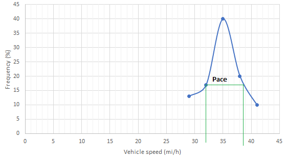
The pace is obtained from the frequency distribution curve above as 32 to 39 mi/h.
After an increase in speed enforcement activities:
The speed ranges from 20 to 37 mi/h giving a speed range of 17. For six classes, the range per class is 2.83 mi/h. A frequency distribution table can then be prepared, as shown below in which the speed classes are listed in column 1 and the mid-values are in column 2. The number of observations for each class is listed in column 3 and the cumulative percentages of all observations are listed in column 6.
| 1 | 2 | 3 | 4 | 5 | 6 | 7 |
| Speed class (mi/h) | Class mid-value | Class frequency, | Percentage of class frequency | Cumulative percentage of class frequency | ||
| 20-22 | 21 | 6 | 126 | 20 | 20 | 253.5 |
| 23-25 | 24 | 8 | 192 | 27 | 47 | 98 |
| 26-28 | 27 | 4 | 108 | 13 | 60 | 1 |
| 29-31 | 30 | 3 | 90 | 10 | 70 | 18.75 |
| 32-34 | 33 | 5 | 165 | 17 | 87 | 151.25 |
| 35-37 | 36 | 4 | 144 | 13 | 100 | 289 |
| Total | 30 | 825 | 811.5 |
Below Figure shows the frequency histogram for the data shown in above Table. The values in columns 2 and 3 of Table are used to draw the frequency histogram, where the abscissa represents the speeds and the ordinate the observed frequency in each class.

Below Figure shows the cumulative frequency distribution curve for the data given. In this case, the cumulative percentages in column 6 of above Table are plotted against the upper limit of each corresponding speed class. This curve gives the percentage of vehicles that are traveling at or below a given speed.

Below figure shows the frequency distribution curve for the data given. In this case, a curve showing percentage of observations against speed is drawn by plotting values from column 5 of above Table against the corresponding values in column 2. The total area under this curve is one or 100 percent.
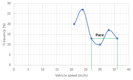
The pace is obtained from the frequency distribution curve drawn above as 27 to 36 mi/h.
Conclusion:
The pace for each set of data are 32 to 39 mi/h and 27 to 36 mi/h respectively.
Want to see more full solutions like this?
Chapter 4 Solutions
Traffic And Highway Engineering


- Why is it important for construction project managers to be flexible when dealing with the many variable factors that pop up in a project?arrow_forwardWhat are some reasons for why a company would accelerate a construction project?arrow_forwardFor the design of a shallow foundation, given the following: Soil: ' = 20° c' = 52 kN/m² Unit weight, y = 15 kN/m³ Modulus of elasticity, E, = 1400 kN/m² Poisson's ratio, μs = 0.35 Foundation: L=2m B=1m Df = 1 m Calculate the ultimate bearing capacity. Use the equation: 1 - qu = c' NcFcs Fcd Fcc +qNqFqsFqdFqc + ½√BN√Fãs F√dƑxc 2 For '=20°, Nc = 14.83, N₁ = 6.4, and N₁ = 5.39. (Enter your answer to three significant figures.) qu = kN/m²arrow_forward
- A 2.0 m wide strip foundation carries a wall load of 350 kN/m in a clayey soil where y = 15 kN/m³, c' = 5.0 kN/m² and ' = 23°. The foundation depth is 1.5 m. For ' = 23°: Nc = 18.05; N₁ = 8.66; Ny = = = 8.20. Determine the factor of safety using the equation below. qu= c' NcFcs FcdFci+qNqFqsFq 1 F + gd. 'qi 2 ·BN√· FF γί Ysyd F (Enter your answer to three significant figures.) FS =arrow_forward2P -1.8 m- -1.8 m- -B Wo P -1.8 m- Carrow_forwardPart F: Progressive activity week 7 Q.F1 Pick the rural location of a project site in Victoria, and its catchment area-not bigger than 25 sqkm, and given the below information, determine the rainfall intensity for ARI 5, 50, 100 year storm event. Show all the details of the procedure. Each student must propose different length of streams and elevations. Use fig below as a sample only. Pt. E-nt 950 200 P: D-40, PC-92.0 300m 300m 000m PL.-02.0 500m HI-MAGO PLA-M 91.00 To be deemed satisfactory the solution must include: Q.F1.1.Choice of catchment location Q.F1.2. A sketch displaying length of stream and elevation Q.F1.3. Catchment's IFD obtained from the Buro of Metheorology for specified ARI Q.F1.4.Calculation of the time of concentration-this must include a detailed determination of the equivalent slope. Q.F1.5.Use must be made of the Bransby-Williams method for the determination of the equivalent slope. Q.F1.6.The graphical display of the estimation of intensities for ARI 5,50, 100…arrow_forward
- I need help finding: -The axial deflection pipe in inches. -The lateral deflection of the beam in inches -The total deflection of the beam like structure in inches ?arrow_forwardA 2.0 m wide strip foundation carries a wall load of 350 kN/m in a clayey soil where y = 17 kN/m³, c' = 5.0 kN/m² and 23°. The foundation depth is 1.5 m. For o' = 23°: Nc = 18.05; N = 8.66; N = 8.20. Determine the factor of safety using the equation below. 1 qu = c' NcFcs Fed Fci +qNqFqs FqdFqi + ½ BN F√s 1 2 (Enter your answer to three significant figures.) s Fyd Fi FS =arrow_forward1.2 m BX B 70 kN.m y = 16 kN/m³ c' = 0 6'-30° Water table Ysat 19 kN/m³ c' 0 &' = 30° A square foundation is shown in the figure above. Use FS = 6, and determine the size of the foundation. Use the Prakash and Saran theory (see equation and figures below). Suppose that F = 450 kN. Qu = BL BL[c′Nc(e)Fcs(e) + qNg(e)Fcs(e) + · 1 YBN(e) F 2 7(e) Fra(e)] (Enter your answer to two significant figures.) B: m Na(e) 60 40- 20- e/B=0 0.1 0.2 0.3 .0.4 0 0 10 20 30 40 Friction angle, ' (deg) Figure 1 Variation of Na(e) with o' Ny(e) 60 40 20 e/B=0 0.3 0.1 0.2 0.4 0 0 10 20 30 40 Friction angle, ' (deg) Figure 2 Variation of Nye) with o'arrow_forward
- K/S 46. (O المهمات الجديدة 0 المنتهية 12 المغـ ۱۱:۰۹ search ليس لديك اي مهمات ☐ ○ ☑arrow_forwardI need help setti if this problem up and solving. I keep doing something wrong.arrow_forward1.0 m (Eccentricity in one direction only)=0.15 m Call 1.5 m x 1.5m Centerline An eccentrically loaded foundation is shown in the figure above. Use FS of 4 and determine the maximum allowable load that the foundation can carry if y = 18 kN/m³ and ' = 35°. Use Meyerhof's effective area method. For '=35°, N = 33.30 and Ny = 48.03. (Enter your answer to three significant figures.) Qall = kNarrow_forward
 Traffic and Highway EngineeringCivil EngineeringISBN:9781305156241Author:Garber, Nicholas J.Publisher:Cengage Learning
 Residential Construction Academy: House Wiring (M...Civil EngineeringISBN:9781285852225Author:Gregory W FletcherPublisher:Cengage Learning
 Engineering Fundamentals: An Introduction to Engi...Civil EngineeringISBN:9781305084766Author:Saeed MoaveniPublisher:Cengage Learning