Determinants of demand and it relevance to the equilibrium position.
Explanation of Solution
Transaction demand for money is the need for money to meet the day-to-day expenditures. It varies directly with nominal
Asset demand for money refers to the desire of public to hold money in the form of financial assets, such as stocks, bonds and so forth. If the interest rate is greater, then people would be interested to save more thereby the asset demand for money would be lower and vice versa. Thus interest rate is the major determinant of the asset demand for money.
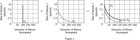
In figure -1, the horizontal axis measures quantity demanded and vertical axis measures the interest rate. The transaction demand for money, represented as Dt, is dependent only on the nominal GDP and has little effect by interest rate, so graphically it is depicted by a vertical line.
The asset demand for money, represented as Da in the figure has an inverse relation with the interest rate since it involves in the
The Total Money demand is the sum of Transaction demand and Asset demand for money
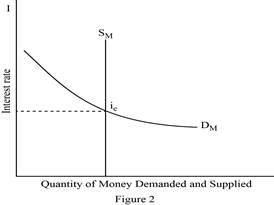
Figure- 2 depicts the equilibrium market, with quantity demanded and supplied measured in the horizontal axis and interest rate in the vertical axis.
The Monetary Authority (usually, the Central Bank of a country) decides on the Money Supply which is unaffected by the decisions that holds money for transaction or as financial asset. The Money Supply (Sm) is depicted by a vertical straight line which is independent of the rate of interest.
The Total Money demand (Dm) depends on the level of income and interest rate. It can be depicted as a linear function of income and interest rate. Demand for money varies directly with levels of income and inversely with the interest rate and slopes downward.
Dm = aY – bi
A
Dm = Sm
The interest rate at which equilibrium is made is the equilibrium interest rate (ie). Thus ie is determined at the point where Dm =Sm.
Let’s now illustrate the effect on equilibrium interest rate due to an increase in the total demand for money.
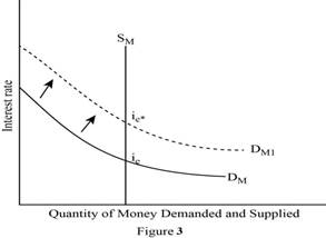
In Figure -3, the horizontal axis measures the quantity of money demanded and supplied and vertical axis represents the interest rate. When the Total money demand increases (shifts to right from DM to DM1) with money supply (SM) remaining constant, the equilibrium interest rate goes up from ie to ie*.
As the money demand increases, the previous interest rate is no longer sustainable because when the demand for money increases it exceeds the supply of money at the previous interest rate. This limits the money available to borrowers or creditors. Also there would be an upward pressure on the interest rate. Thus previous interest rate is no longer maintainable.
Concept Introduction:
Transaction demand for money: It refers to that amount of money required by individuals or firms to finance their current transaction or forthcoming expenditure.
Asset demand for money: It is the extent to which, people hold money in the form of asset.
Total Money demand: It refers to the desire of individuals or firms to hold money in the form of both financial assets and for transactions at each possible interest rate.
Equilibrium Interest rate: It is the point in which demand for money equals with the supply of money.
Want to see more full solutions like this?
Chapter 34 Solutions
EBK ECONOMICS

- PART II: Multipart Problems wood or solem of triflussd aidi 1. Assume that a society has a polluting industry comprising two firms, where the industry-level marginal abatement cost curve is given by: MAC = 24 - ()E and the marginal damage function is given by: MDF = 2E. What is the efficient level of emissions? b. What constant per-unit emissions tax could achieve the efficient emissions level? points) c. What is the net benefit to society of moving from the unregulated emissions level to the efficient level? In response to industry complaints about the costs of the tax, a cap-and-trade program is proposed. The marginal abatement cost curves for the two firms are given by: MAC=24-E and MAC2 = 24-2E2. d. How could a cap-and-trade program that achieves the same level of emissions as the tax be designed to reduce the costs of regulation to the two firms?arrow_forwardOnly #4 please, Use a graph please if needed to help provearrow_forwarda-carrow_forward
- For these questions, you must state "true," "false," or "uncertain" and argue your case (roughly 3 to 5 sentences). When appropriate, the use of graphs will make for stronger answers. Credit will depend entirely on the quality of your explanation. 1. If the industry facing regulation for its pollutant emissions has a lot of political capital, direct regulatory intervention will be more viable than an emissions tax to address this market failure. 2. A stated-preference method will provide a measure of the value of Komodo dragons that is more accurate than the value estimated through application of the travel cost model to visitation data for Komodo National Park in Indonesia. 3. A correlation between community demographics and the present location of polluting facilities is sufficient to claim a violation of distributive justice. olsvrc Q 4. When the damages from pollution are uncertain, a price-based mechanism is best equipped to manage the costs of the regulator's imperfect…arrow_forwardFor environmental economics, question number 2 only please-- thank you!arrow_forwardFor these questions, you must state "true," "false," or "uncertain" and argue your case (roughly 3 to 5 sentences). When appropriate, the use of graphs will make for stronger answers. Credit will depend entirely on the quality of your explanation. 1. If the industry facing regulation for its pollutant emissions has a lot of political capital, direct regulatory intervention will be more viable than an emissions tax to address this market failure. cullog iba linevoz ve bubivorearrow_forward
- Exercise 3 The production function of a firm is described by the following equation Q=10,000-3L2 where L stands for the units of labour. a) Draw a graph for this equation. Use the quantity produced in the y-axis, and the units of labour in the x-axis. b) What is the maximum production level? c) How many units of labour are needed at that point? d) Provide one reference with you answer.arrow_forwardExercise 1 Consider the market supply curve which passes through the intercept and from which the market equilibrium data is known, this is, the price and quantity of equilibrium PE=50 and QE=2000. Considering those two points, find the equation of the supply. Draw a graph of this line. Provide one reference with your answer. Exercise 2 Considering the previous supply line, determine if the following demand function corresponds to the market demand equilibrium stated above. QD=3000-2p.arrow_forwardConsider the market supply curve which passes through the intercept and from which the marketequilibrium data is known, this is, the price and quantity of equilibrium PE=50 and QE=2000.a. Considering those two points, find the equation of the supply. b. Draw a graph of this line.arrow_forward
- Government Purchases and Tax Revenues A B GDP T₂ Refer to the diagram. Discretionary fiscal policy designed to slow the economy is illustrated by Multiple Choice the shift of curve T₁ to T2. a movement from d to balong curve T₁.arrow_forwardSection III: Empirical Findings: Descriptive Statistics and inferential statistics………………..40% Descriptive statistics provide details about the Y variable, based on the sample for the 10-year period. Here, you use Excell or manually compute Mean or the average income per capita. Interpret the meaning of average income per capita. Draw the line chart showing the educational performance over the time-period of your study. Label the Vertical axis as Y performance and X axis as the explanatory variable (X1) . Do the same thing between Y and X2 Empirical/ Inferential Statistics: Here, use the sample information to perform the following: Draw the Scatter plot and impose the trend line: showing the Y variable and explanatory variables ( X1). Draw the scatter plot and impose the tend line: Showing Y and X2. Does your evidence (data) support your theory? Refer to the trend line: Is the relationship positive or negative as expected? Based on the data sheet below: Years Y ( per…arrow_forwardSection III: Empirical Findings: Descriptive Statistics and inferential statistics………………..40% Descriptive statistics provide details about the Y variable, based on the sample for the 10-year period. Here, you use Excell or manually compute Mean or the average income per capita. Interpret the meaning of average income per capita. Draw the line chart showing the educational performance over the time-period of your study. Label the Vertical axis as Y performance and X axis as the explanatory variable (X1) . Do the same thing between Y and X2 Empirical/ Inferential Statistics: Here, use the sample information to perform the following: Draw the Scatter plot and impose the trend line: showing the Y variable and explanatory variables ( X1). Draw the scatter plot and impose the tend line: Showing Y and X2. Does your evidence (data) support your theory? Refer to the trend line: Is the relationship positive or negative as expected? Create graphs based on table below; Years Y ( per…arrow_forward


 Economics (MindTap Course List)EconomicsISBN:9781337617383Author:Roger A. ArnoldPublisher:Cengage Learning
