Chapter 31, Problem 12P

To determine

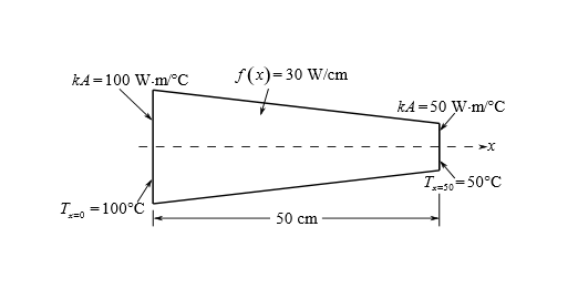
To calculate: The temperature distribution in a rod as shown in figure below with internal heat generation using the finite-element method and also derive the element nodal equations using Fourier heat conduction.

Answer to Problem 12P

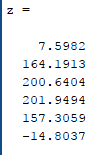
Solution: The temperature distribution in a rod at various nodes is shown below,

Explanation of Solution

Given Information:

To develop nodal equations for the temperature and their gradients at each of the six nodes. The element nodal equations is given as,

$q_k=-kA\frac{dT}{\partial x}$

With the heat conservation relationships is,

${\displaystyle \sum \left[q_k+f\left(x\right)\right]}=0$

Here,

$\begin{array}{c}{q}_k=\text{heat flow}\left(\text{W}\right)\\ k=\text{thermal conductivity}\left(\frac{\text{W}}{\text{m}{\cdot }^{\text{o}}\text{C}}\right)\\ A=\text{cross-sectional area}\left({\text{m}}^{\text{2}}\right)\\ f\left(x\right)=\text{heat source}\left(\frac{\text{W}}{\text{cm}}\right)\end{array}$

The given rod is 50 cm long, the x-coordinate is positive to the right end and zero at the left end, $kA=100$ and $5\text{0 Wm/°C}$ at $x=0$ and at $x=50$ respectively. The given data are,

$\begin{array}{l}kA=100,f\left(x\right)=3\text{0 }\frac{\text{W}}{\text{cm}}\\ T{|}_{x=0}={100}^{\text{ o}}\text{C, }T{|}_{x=50}={\text{50 }}^{\text{o}}\text{C}\end{array}$

Calculation:

The element 1 the equations for the node 1 and node 2 is,

Solve the equation for node 1,

$\begin{array}{c}{\displaystyle \sum q_k}+f\left(x\right)=0\\ \left(-kA\frac{dT}{dx}{|}_1+kA\left(\frac{1}{x_2-x_1}\right)\left(T_2-T_1\right)\right)+{\displaystyle {\int }_{x_1}^{x_2}{N}_1\cdot f\left(x\right)\cdot dx}=0\\ \left(-kA\frac{dT}{dx}{|}_1+kA\left(\frac{1}{x_2-x_1}\right)\left(T_2-T_1\right)\right)+{\displaystyle {\int }_{x_1}^{x_2}\left(\frac{x_2-x}{x_2-x_1}\right)\cdot f\left(x\right)\cdot dx}=0\end{array}$

Substitute the value from given data,

$\begin{array}{c}\left(-\left(100\right)\frac{dT}{dx}{|}_1+\left(\frac{95}{10}\right)\left(T_2-T_1\right)\right)+{\displaystyle {\int }_0^{10}\left(\frac{10-x}{10-0}\right)\cdot 30\cdot dx}=0\\ \left(-\left(100\right)\frac{dT}{dx}{|}_1+9.5\left(T_2-T_1\right)\right)+3{\left[10x-\frac{x^2}{2}\right]}_0^{10}=0\end{array}$

Change the temperature so the equation becomes,

$9.5\left(T_1-T_2\right)=-\left(100\right)\frac{dT}{dx}{|}_1+150$

Solve the equation for the node 2,

$\begin{array}{c}{\displaystyle \sum q_k}+f\left(x\right)=0\\ \left(-kA\frac{dT}{dx}{|}_2+kA\left(\frac{1}{x_2-x_1}\right)\left(T_2-T_1\right)\right)+{\displaystyle {\int }_{x_1}^{x_2}{N}_2\cdot f\left(x\right)\cdot dx}=0\\ \left(-kA\frac{dT}{dx}{|}_2+kA\left(\frac{1}{x_2-x_1}\right)\left(T_2-T_1\right)\right)+{\displaystyle {\int }_{x_1}^{x_2}\left(\frac{x-x_2}{x_2-x_1}\right)\cdot f\left(x\right)\cdot dx}=0\end{array}$

Substitute the values from given data,

$\begin{array}{c}\left(90\frac{dT}{dx}{|}_1+\left(\frac{95}{10}\right)\left(T_2-T_1\right)\right)+{\displaystyle {\int }_0^{10}\left(\frac{x-0}{10-0}\right)\cdot 30\cdot dx}=0\\ \left(90\frac{dT}{dx}{|}_2+9.5\left(T_2-T_1\right)\right)+3{\left[\frac{x^2}{2}\right]}_0^{10}=0\\ \left(90\frac{dT}{dx}{|}_2+9.5\left(T_2-T_1\right)\right)+3\left[\frac{100}{2}\right]=0\\ \left(90\frac{dT}{dx}{|}_2+9.5\left(T_2-T_1\right)\right)+150=0\end{array}$

So, the equation of node 2 is,

$-9.5\left(T_2-T_1\right)=90\frac{dT}{dx}{|}_2+150$

Similarly, the value for other nodes is calculated. For element 2 at node 2,

$\begin{array}{c}{\displaystyle \sum q_k}+f\left(x\right)=0\\ \left(-kA\frac{dT}{dx}{|}_2+kA\left(\frac{1}{x_2-x_1}\right)\left(T_3-T_2\right)\right)+{\displaystyle {\int }_{x_1}^{x_2}{N}_1\cdot f\left(x\right)\cdot dx}=0\\ \left(-kA\frac{dT}{dx}{|}_2+kA\left(\frac{1}{x_2-x_1}\right)\left(T_3-T_2\right)\right)+{\displaystyle {\int }_{x_1}^{x_2}\left(\frac{x_2-x}{x_2-x_1}\right)\cdot f\left(x\right)\cdot dx}=0\end{array}$

Substitute the values from given data,

$\begin{array}{c}\left(-90\frac{dT}{dx}{|}_2+\left(\frac{85}{10}\right)\left(T_3-T_2\right)\right)+{\displaystyle {\int }_0^{10}\left(\frac{10-x}{10-0}\right)\cdot 30\cdot dx}=0\\ \left(-\left(90\right)\frac{dT}{dx}{|}_2+8.5\left(T_3-T_2\right)\right)+3{\left[10x-\frac{x^2}{2}\right]}_0^{10}=0\\ \left(-90\frac{dT}{dx}{|}_2+8.5\left(T_3-T_2\right)\right)+3\left[50\right]=0\\ \left(-\left(90\right)\frac{dT}{dx}{|}_2+8.5\left(T_3-T_2\right)\right)+150=0\end{array}$

Change the state so the equation becomes,

$8.5\left(T_2-T_3\right)=-90\frac{dT}{dx}{|}_2+150$

Derive for node 3,

$\begin{array}{c}{\displaystyle \sum q_k}+f\left(x\right)=0\\ \left(-kA\frac{dT}{dx}{|}_3+kA\left(\frac{1}{x_2-x_1}\right)\left(T_2-T_3\right)\right)+{\displaystyle {\int }_{x_1}^{x_2}{N}_2\cdot f\left(x\right)\cdot dx}=0\\ \left(-kA\frac{dT}{dx}{|}_3+kA\left(\frac{1}{x_2-x_1}\right)\left(T_2-T_3\right)\right)+{\displaystyle {\int }_{x_1}^{x_2}\left(\frac{x-x_2}{x_2-x_1}\right)\cdot f\left(x\right)\cdot dx}=0\end{array}$

Substitute the values from given data,

$\begin{array}{c}\left(80\frac{dT}{dx}{|}_3+\left(\frac{85}{10}\right)\left(T_2-T_3\right)\right)+{\displaystyle {\int }_0^{10}\left(\frac{x-0}{10-0}\right)\cdot 30\cdot dx}=0\\ \left(80\frac{dT}{dx}{|}_3+8.5\left(T_2-T_3\right)\right)+3{\left[\frac{x^2}{2}\right]}_0^{10}=0\\ \left(80\frac{dT}{dx}{|}_3+8.5\left(T_2-T_3\right)\right)+3\left[\frac{100}{2}\right]=0\\ \left(80\frac{dT}{dx}{|}_3+8.5\left(T_2-T_3\right)\right)+150=0\end{array}$

So, the equation of node 3 is,

$-8.5\left(T_2-T_3\right)=80\frac{dT}{dx}{|}_3+150$

Derive the equation for the element 3,

Node 3

$\begin{array}{c}{\displaystyle \sum q_k}+f\left(x\right)=0\\ \left(-kA\frac{dT}{dx}{|}_3+kA\left(\frac{1}{x_2-x_1}\right)\left(T_3-T_4\right)\right)+{\displaystyle {\int }_{x_1}^{x_2}{N}_1\cdot f\left(x\right)\cdot dx}=0\\ \left(-kA\frac{dT}{dx}{|}_3+kA\left(\frac{1}{x_2-x_1}\right)\left(T_3-T_4\right)\right)+{\displaystyle {\int }_{x_1}^{x_2}\left(\frac{x_2-x}{x_2-x_1}\right)\cdot f\left(x\right)\cdot dx}=0\end{array}$

Substitute the values from given data,

$\begin{array}{c}\left(-80\frac{dT}{dx}{|}_3+\left(\frac{75}{10}\right)\left(T_3-T_4\right)\right)+{\displaystyle {\int }_0^{10}\left(\frac{10-x}{10-0}\right)\cdot 30\cdot dx}=0\\ \left(-80\frac{dT}{dx}{|}_3+7.5\left(T_3-T_4\right)\right)+3{\left[10x-\frac{x^2}{2}\right]}_0^{10}=0\\ \left(-80\frac{dT}{dx}{|}_3+7.5\left(T_3-T_4\right)\right)+3\left[50\right]=0\\ \left(-\left(80\right)\frac{dT}{dx}{|}_3+7.5\left(T_3-T_4\right)\right)+150=0\end{array}$

Change the state so the equation becomes,

$7.5\left(T_3-T_4\right)=-80\frac{dT}{dx}{|}_3+150$

Derive for node 4,

$\begin{array}{c}{\displaystyle \sum q_k}+f\left(x\right)=0\\ \left(-kA\frac{dT}{dx}{|}_4+kA\left(\frac{1}{x_2-x_1}\right)\left(T_3-T_4\right)\right)+{\displaystyle {\int }_{x_1}^{x_2}{N}_2\cdot f\left(x\right)\cdot dx}=0\\ \left(-kA\frac{dT}{dx}{|}_4+kA\left(\frac{1}{x_2-x_1}\right)\left(T_3-T_4\right)\right)+{\displaystyle {\int }_{x_1}^{x_2}\left(\frac{x-x_2}{x_2-x_1}\right)\cdot f\left(x\right)\cdot dx}=0\end{array}$

Substitute the values from given data,

$\begin{array}{c}\left(70\frac{dT}{dx}{|}_4+\left(\frac{75}{10}\right)\left(T_3-T_4\right)\right)+{\displaystyle {\int }_0^{10}\left(\frac{x-0}{10-0}\right)\cdot 30\cdot dx}=0\\ \left(70\frac{dT}{dx}{|}_4+7.5\left(T_3-T_4\right)\right)+3{\left[\frac{x^2}{2}\right]}_0^{10}=0\\ \left(70\frac{dT}{dx}{|}_4+7.5\left(T_3-T_4\right)\right)+3\left[\frac{100}{2}\right]=0\\ \left(70\frac{dT}{dx}{|}_4+7.5\left(T_3-T_4\right)\right)+150=0\end{array}$

So, the equation of node 4 is,

$-7.5\left(T_3-T_4\right)=70\frac{dT}{dx}{|}_4+150$

Derive the equation for the element 4,

The equations for node 4 is,

$\begin{array}{c}{\displaystyle \sum q_k}+f\left(x\right)=0\\ \left(-kA\frac{dT}{dx}{|}_4+kA\left(\frac{1}{x_2-x_1}\right)\left(T_5-T_4\right)\right)+{\displaystyle {\int }_{x_1}^{x_2}{N}_1\cdot f\left(x\right)\cdot dx}=0\\ \left(-kA\frac{dT}{dx}{|}_4+kA\left(\frac{1}{x_2-x_1}\right)\left(T_5-T_4\right)\right)+{\displaystyle {\int }_{x_1}^{x_2}\left(\frac{x_2-x}{x_2-x_1}\right)\cdot f\left(x\right)\cdot dx}=0\end{array}$

Substitute the values from given data,

$\begin{array}{c}\left(-70\frac{dT}{dx}{|}_4+\left(\frac{65}{10}\right)\left(T_5-T_4\right)\right)+{\displaystyle {\int }_0^{10}\left(\frac{10-x}{10-0}\right)\cdot 30\cdot dx}=0\\ \left(-70\frac{dT}{dx}{|}_4+6.5\left(T_5-T_4\right)\right)+3{\left[10x-\frac{x^2}{2}\right]}_0^{10}=0\\ \left(-70\frac{dT}{dx}{|}_4+6.5\left(T_5-T_4\right)\right)+3\left[50\right]=0\\ \left(-\left(70\right)\frac{dT}{dx}{|}_4+6.5\left(T_5-T_4\right)\right)+150=0\end{array}$

Change the state so the equation becomes,

$6.5\left(T_4-T_5\right)=-70\frac{dT}{dx}{|}_4+150$

Derive the equation for the node 5,

$\begin{array}{c}{\displaystyle \sum q_k}+f\left(x\right)=0\\ \left(-kA\frac{dT}{dx}{|}_5+kA\left(\frac{1}{x_2-x_1}\right)\left(T_4-T_5\right)\right)+{\displaystyle {\int }_{x_1}^{x_2}{N}_2\cdot f\left(x\right)\cdot dx}=0\\ \left(-kA\frac{dT}{dx}{|}_5+kA\left(\frac{1}{x_2-x_1}\right)\left(T_4-T_5\right)\right)+{\displaystyle {\int }_{x_1}^{x_2}\left(\frac{x-x_2}{x_2-x_1}\right)\cdot f\left(x\right)\cdot dx}=0\end{array}$

Substitute the values from given data,

$\begin{array}{c}\left(60\frac{dT}{dx}{|}_5+\left(\frac{65}{10}\right)\left(T_4-T_5\right)\right)+{\displaystyle {\int }_0^{10}\left(\frac{x-0}{10-0}\right)\cdot 30\cdot dx}=0\\ \left(60\frac{dT}{dx}{|}_5+6.5\left(T_4-T_5\right)\right)+3{\left[\frac{x^2}{2}\right]}_0^{10}=0\\ \left(60\frac{dT}{dx}{|}_5+6.5\left(T_4-T_5\right)\right)+3\left[\frac{100}{2}\right]=0\\ \left(60\frac{dT}{dx}{|}_5+6.5\left(T_4-T_5\right)\right)+150=0\end{array}$

So, the equation of node 5 is,

$-6.5\left(T_3-T_4\right)=60\frac{dT}{dx}{|}_5+150$

Derive the equation for the element 5,

For node 5,

$\begin{array}{c}{\displaystyle \sum q_k}+f\left(x\right)=0\\ \left(-kA\frac{dT}{dx}{|}_5+kA\left(\frac{1}{x_2-x_1}\right)\left(T_6-T_5\right)\right)+{\displaystyle {\int }_{x_1}^{x_2}{N}_1\cdot f\left(x\right)\cdot dx}=0\\ \left(-kA\frac{dT}{dx}{|}_5+kA\left(\frac{1}{x_2-x_1}\right)\left(T_6-T_5\right)\right)+{\displaystyle {\int }_{x_1}^{x_2}\left(\frac{x_2-x}{x_2-x_1}\right)\cdot f\left(x\right)\cdot dx}=0\end{array}$

Substitute the values from given data,

$\begin{array}{c}\left(-60\frac{dT}{dx}{|}_5+\left(\frac{55}{10}\right)\left(T_6-T_5\right)\right)+{\displaystyle {\int }_0^{10}\left(\frac{10-x}{10-0}\right)\cdot 30\cdot dx}=0\\ \left(-60\frac{dT}{dx}{|}_4+5.5\left(T_6-T_5\right)\right)+3{\left[10x-\frac{x^2}{2}\right]}_0^{10}=0\\ \left(-60\frac{dT}{dx}{|}_4+5.5\left(T_6-T_5\right)\right)+3\left[50\right]=0\\ \left(-\left(60\right)\frac{dT}{dx}{|}_4+5.5\left(T_6-T_5\right)\right)+150=0\end{array}$

Change the state so the equation becomes,

$5.5\left(T_5-T_6\right)=-60\frac{dT}{dx}{|}_5+150$

Derive the equation for node 6,

$\begin{array}{c}{\displaystyle \sum q_k}+f\left(x\right)=0\\ \left(-kA\frac{dT}{dx}{|}_6+kA\left(\frac{1}{x_2-x_1}\right)\left(T_5-T_6\right)\right)+{\displaystyle {\int }_{x_1}^{x_2}{N}_2\cdot f\left(x\right)\cdot dx}=0\\ \left(-kA\frac{dT}{dx}{|}_6+kA\left(\frac{1}{x_2-x_1}\right)\left(T_5-T_6\right)\right)+{\displaystyle {\int }_{x_1}^{x_2}\left(\frac{x-x_2}{x_2-x_1}\right)\cdot f\left(x\right)\cdot dx}=0\end{array}$

Substitute the values from given data,

$\begin{array}{c}\left(50\frac{dT}{dx}{|}_6+\left(\frac{55}{10}\right)\left(T_5-T_6\right)\right)+{\displaystyle {\int }_0^{10}\left(\frac{x-0}{10-0}\right)\cdot 30\cdot dx}=0\\ \left(50\frac{dT}{dx}{|}_5+5.5\left(T_5-T_6\right)\right)+3{\left[\frac{x^2}{2}\right]}_0^{10}=0\\ \left(50\frac{dT}{dx}{|}_5+5.5\left(T_5-T_6\right)\right)+3\left[\frac{100}{2}\right]=0\\ \left(50\frac{dT}{dx}{|}_5+5.5\left(T_5-T_6\right)\right)+150=0\end{array}$

So, the equation of node 6 is,

$-5.5\left(T_5-T_6\right)=50\frac{dT}{dx}{|}_5+150$

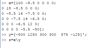
The equation assembly is given as,

$\left[\begin{array}{cccccc}9.5& -9.5& & & & \\ -9.5& 18& -8.5& & & \\ & -8.5& 16& -7.5& & \\ & & -7.5& 14& -6.5& \\ & & & -6.5& 12& -5.5\\ & & & & -5.5& 5.5\end{array}\right]\left[\begin{array}{c}{T}_1\\ T_2\\ T_3\\ T_4\\ T_5\\ T_6\end{array}\right]=\left\{\begin{array}{c}-100\frac{dT}{dx}{|}_1+150\\ 300\\ 300\\ 300\\ 300\\ 50\frac{dT}{dx}{|}_6+150\end{array}\right\}$

Insert the boundary conditions then the matrix becomes,

$\left[\begin{array}{cccccc}100& -9.5& & & & \\ & 18& -8.5& & & \\ & -8.5& 16& -7.5& & \\ & & -7.5& 14& -6.5& \\ & & & -6.5& 12& 0\\ & & & & -5.5& -50\end{array}\right]\left[\begin{array}{c}\frac{dT}{dx}{|}_1\\ T_2\\ T_3\\ T_4\\ T_5\\ \frac{dT}{dx}{|}_6\end{array}\right]=\left\{\begin{array}{c}-800\\ 1250\\ 300\\ 300\\ 575\\ -125\end{array}\right\}$

Use MATLAB to write code for solving the matrix,

The desired output is,