Subpart (a):
Effect on Aggregate Demand and Supply.
Subpart (a):
Explanation of Solution
When consumers fear of an impending economic depression, their spending decline and they tend to save more. This leads to a decrease in AD curve. This can be explained by using figure 1.
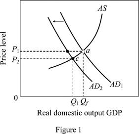
In figure 1, horizontal axis represents the real GDP(
Concept Introduction:
Aggregate demand (AD): Aggregate demand refers to the total value of the goods and services that are demanded at a particular price in a given period of time.
Subpart (b):
Effect on Aggregate Demand and Supply.
Subpart (b):
Explanation of Solution
When a new tax is imposed on producers, cost of production comes up and there is no incentive to produce more. This leads to a decline in
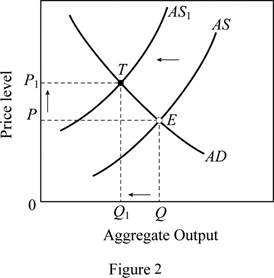
In figure 2, horizontal axis represents the real GDP and vertical axis represents price level. In this case, the AS curve shifts left (from AS to AS1), this moves the equilibrium position from E to T, thus there is a decline in the output (from Q to Q1) and a rise in the price level (from P to P1).
Concept Introduction:
Aggregate demand (AD): Aggregate demand refers to the total value of the goods and services that are demanded at a particular price in a given period of time.
Aggregate supply (AS): Aggregate supply refers to the total value of the goods and services that are available for purchase at a particular price in a given period of time.
Subpart (c):
Effect on Aggregate Demand and Supply.
Subpart (c):
Explanation of Solution
Figure 3 can explain the shift in AD curve due to reduction in interest rates at each price level. In figure 3, horizontal axis measures the real GDP and vertical axis measures the price level.
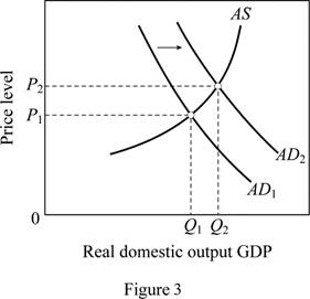
A reduction in interest rates decreases the borrowing cost increases the spending.
This leads to a rightward shift of AD curve from AD1 to AD2. Thus, it brings the output and price level up. The output increases from Q1 to Q2 and price level increases from P1 to P2.
Concept Introduction:
Aggregate demand (AD): Aggregate demand refers to the total value of the goods and services that are demanded at a particular price in a given period of time.
Aggregate supply (AS): Aggregate supply refers to the total value of the goods and services that are available for purchase at a particular price in a given period of time.
Subpart (d):
Effect on Aggregate Demand and Supply.
Subpart (d):
Explanation of Solution
A major increase in spending shifts the AD curve to right. Figure 4 is used to explain this situation. In figure 4, horizontal axis measures the real GDP and vertical axis measures the price level.
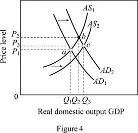
Government expenditure is a key determinant of changes in the aggregate demand. The increase in government spending (spending for health care) increases the aggregate demand leading to a shift of AD curve from AD1 to AD2. Any real improvements in healthcare resulting from the spending would ultimately increase the productivity, thereby shifting the AS curve to the right (from AS1 to AS2). The equilibrium moves from a to c leading to an increase in output (from Q1 to Q3) .It will also move the price level up from P1 to P3.
Concept Introduction:
Aggregate demand (AD): Aggregate demand refers to the total value of the goods and services that are demanded at a particular price in a given period of time.
Aggregate supply (AS): Aggregate supply refers to the total value of the goods and services that are available for purchase at a particular price in a given period of time.
Subpart (e):
Effect on Aggregate Demand and Supply.
Subpart (e):
Explanation of Solution
The general expectation of surging inflation in the near future will increase the aggregate demand today because the consumers will want to buy products before their prices escalate. This can be illustrated using figure 3. As a result, there will be a rightward shift of AD curve from AD1 to AD2 which brings the output and price level up. In figure 3, the output increases from Q1 to Q2 and price level increases from P1 to P2.
Concept Introduction:
Aggregate demand (AD): Aggregate demand refers to the total value of the goods and services that are demanded at a particular price in a given period of time.
Aggregate supply (AS): Aggregate supply refers to the total value of the goods and services that are available for purchase at a particular price in a given period of time.
Subpart (f):
Effect on Aggregate Demand and Supply.
Subpart (f):
Explanation of Solution
Figure 5 is used to explain this case. In figure 5, horizontal axis measures the real GDP and vertical axis measures the price level.
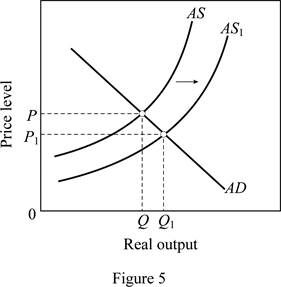
As oil prices fall (oil is an imported resource) due to the disintegration of OPEC, it increases the U.S. aggregate supply. As a result, there will be a rightward shift of AS curve from AS to AS1. This brings the output level up from Q to Q1 and price level down from P to P1.
Concept Introduction:
Aggregate demand (AD): Aggregate demand refers to the total value of the goods and services that are demanded at a particular price in a given period of time.
Aggregate supply (AS): Aggregate supply refers to the total value of the goods and services that are available for purchase at a particular price in a given period of time.
Subpart (g):
Effect on Aggregate Demand and Supply.
Subpart (g):
Explanation of Solution
A reduction in the personal income tax rates raises take-home income increases consumer purchases at each possible price level. This is illustrated in figure 3. Tax cuts shift the aggregate demand curve to the right from AD1 to AD2 which brings the output and price level up. In figure 3, the output increases from Q1 to Q2 and price level increases from P1 to P2.
Concept Introduction:
Aggregate demand (AD): Aggregate demand refers to the total value of the goods and services that are demanded at a particular price in a given period of time.
Aggregate supply (AS): Aggregate supply refers to the total value of the goods and services that are available for purchase at a particular price in a given period of time.
Subpart (h):
Effect on Aggregate Demand and Supply.
Subpart (h):
Explanation of Solution
The sizable increase the labor productivity with no change in nominal wages will increase the overall productivity as more output is available for the given input. This increases the aggregate supply thereby shifting the AS curve to the right from AS to AS1 (Refer Figure 5). This leads to an increase in output (from Q to Q1) and a decrease in price level from P to P1.
Concept Introduction:
Aggregate demand (AD): Aggregate demand refers to the total value of the goods and services that are demanded at a particular price in a given period of time.
Aggregate supply (AS): Aggregate supply refers to the total value of the goods and services that are available for purchase at a particular price in a given period of time.
Subpart (i):
Effect on Aggregate Demand and Supply.
Subpart (i):
Explanation of Solution
This case can be explained using Figure 2. When there is an increase in nominal wages with no change in productivity, it increases per unit cost of production. This force the AS curve to shift left (from AS to AS1). The equilibrium position moves from E to T, thus there are a decline in the output (from Q to Q1) and a rise in the price level (from P to P1).
Concept Introduction:
Aggregate demand (AD): Aggregate demand refers to the total value of the goods and services that are demanded at a particular price in a given period of time.
Aggregate supply (AS): Aggregate supply refers to the total value of the goods and services that are available for purchase at a particular price in a given period of time.
Subpart (j):
Effect on Aggregate Demand and Supply.
Subpart (j):
Explanation of Solution
Figure 6 shows the impact of increasing demand and decreasing supply.
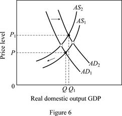
Figure 6 is used to explain this condition. The horizontal axis in Figure 6 measures the real domestic output whereas price level is measured by the vertical axis. A rise in net exports (higher exports relative to imports) shifts the aggregate demand curve to the right (from AD1 to AD2). But, due to the higher input prices, per unit cost is more, leading to a shift of the aggregate supply curve to the left from AS1 to AS2. This leads to an increase in output from Q to Q1 along with an increase in price level from P to P1.
Concept Introduction:
Aggregate demand (AD): Aggregate demand refers to the total value of the goods and services that are demanded at a particular price in a given period of time.
Aggregate supply (AS): Aggregate supply refers to the total value of the goods and services that are available for purchase at a particular price in a given period of time.
Want to see more full solutions like this?
Chapter 30 Solutions
Economics: Principles, Problems, & Policies (McGraw-Hill Series in Economics) - Standalone book

- I need help in seeing how these are the answers. If you could please write down your steps so I can see how it's done please.arrow_forwardSuppose that a random sample of 216 twenty-year-old men is selected from a population and that their heights and weights are recorded. A regression of weight on height yields Weight = (-107.3628) + 4.2552 x Height, R2 = 0.875, SER = 11.0160 (2.3220) (0.3348) where Weight is measured in pounds and Height is measured in inches. A man has a late growth spurt and grows 1.6200 inches over the course of a year. Construct a confidence interval of 90% for the person's weight gain. The 90% confidence interval for the person's weight gain is ( ☐ ☐) (in pounds). (Round your responses to two decimal places.)arrow_forwardSuppose that (Y, X) satisfy the assumptions specified here. A random sample of n = 498 is drawn and yields Ŷ= 6.47 + 5.66X, R2 = 0.83, SER = 5.3 (3.7) (3.4) Where the numbers in parentheses are the standard errors of the estimated coefficients B₁ = 6.47 and B₁ = 5.66 respectively. Suppose you wanted to test that B₁ is zero at the 5% level. That is, Ho: B₁ = 0 vs. H₁: B₁ #0 Report the t-statistic and p-value for this test. Definition The t-statistic is (Round your response to two decimal places) ☑ The Least Squares Assumptions Y=Bo+B₁X+u, i = 1,..., n, where 1. The error term u; has conditional mean zero given X;: E (u;|X;) = 0; 2. (Y;, X¡), i = 1,..., n, are independent and identically distributed (i.i.d.) draws from i their joint distribution; and 3. Large outliers are unlikely: X; and Y, have nonzero finite fourth moments.arrow_forward
- Asap pleasearrow_forwardTasks Exercise 1 Assess the following functions: 1. f(x)= x2+6x+2 2.f '(x)=10x-2x2+5 a. Find the stationary points. (5 marks) b. Determine whether the stationary point is a maximum or minimum. (5 marks) c. Draw the corresponding curves (5 marks)arrow_forwardProblem 2: The sales data over the last 10 years for the Acme Hardware Store are as follows: 2003 $230,000 2008 $526,000 2004 276,000 2009 605,000 2005 328,000 2010 690,000 2006 388,000 2011 779,000 2007 453,000 2012 873,000 1. Calculate the compound growth rate for the period of 2003 to 2012. 2. Based on your answer to part a, forecast sales for both 2013 and 2014. 3. Now calculate the compound growth rate for the period of 2007 to 2012. 1. Based on your answer to part e, forecast sales for both 2013 and 2014. 5. What is the major reason for the differences in your answers to parts b and d? If you were to make your own projections, what would you forecast? (Drawing a graph is very helpful.)arrow_forward
- Exercise 4A firm has the following average cost: AC = 200 + 2Q – 36 Q Find the stationary point and determine if it is a maximum or a minimum.b. Find the marginal cost function.arrow_forwardExercise 4A firm has the following average cost: AC = 200 + 2Q – 36 Q Find the stationary point and determine if it is a maximum or a minimum.b. Find the marginal cost function.arrow_forwardExercise 2A firm has the following short-run production function: Q = 30L2 -0.5L3a. Make a table with two columns: Production and Labour b. Add a third column to the table with the marginal product of labour c. Graph the values that you estimated for the production function and the marginal product oflabour Exercise 3A Firm has the following production function: Q= 20L-0.4L2a. Using differential calculus find the unit of labour that maximizes the production. b. Estimate function of Marginal product of labor c. Obtain the Average product of labor. d. Find the point at which the Marginal Product of Labour is equal to the Average Product of Labour.arrow_forward
- Problem 3 You have the following data for the last 12 months' sales for the PRQ Corporation (in thousands of dollars): January 500 July 610 February 520 August 620 March 520 September 580 April 510 October 550 May 530 November 510 June 580 December 480 1. Calculate a 3-month centered moving average. 2. Use this moving average to forecast sales for January of next year. 3. If you were asked to forecast January and February sales for next year, would you be confident of your forecast using the preceding moving averages? Why or why not? expect? Explain.arrow_forwardProblem 5 The MNO Corporation is preparing for its stockholder meeting on May 15, 2013. It sent out proxies to its stockholders on March 15 and asked stockholders who plan to attend the meeting to respond. To plan for a sufficient number of information packages to be distributed at the meeting, as well as for refreshments to be served, the company has asked you to forecast the number of attending stockholders. By April 15, 378 stockholders have expressed their intention to attend. You have available the following data for the last 6 years for total attendance at the stockholder meeting and the number of positive responses as of April 15: Year Positive Responses Attendance 2007 322 520 2008 301 550 2009 398 570 2010 421 600 2011 357 570 2012 452 650 1. What is your attendance forecast for the 2013 stockholder meeting? 2. Are there any other factors that could affect attendance, and thus make your forecast inac- curate?arrow_forwardProblem 4 Office Enterprises (OE) produces a line of metal office file cabinets. The company's economist, having investigated a large number of past data, has established the following equation of demand for these cabinets: Q=10,000+6013-100P+50C Q=Annual number of cabinets sold B = Index of nonresidential construction P = Average price per cabinet charged by OE C=Average price per cabinet charged by OE's closest competitor It is expected that next year's nonresidential construction index will stand at 160, OE's average price will be $40, and the competitor's average price will be $35. 1. Forecast next year's sales. 2. What will be the effect if the competitor lowers its price to 832? If it raises its price to $36? 3. What will happen if OE reacts to the decrease mentioned in part b by lowering its price to $37? 4. If the index forecast was wrong, and it turns out to be only 140 next year, what will be the effect on OE's sales? If not, what does it measure?arrow_forward
 Essentials of Economics (MindTap Course List)EconomicsISBN:9781337091992Author:N. Gregory MankiwPublisher:Cengage Learning
 Principles of Economics (MindTap Course List)EconomicsISBN:9781305585126Author:N. Gregory MankiwPublisher:Cengage Learning
 Principles of Macroeconomics (MindTap Course List)EconomicsISBN:9781285165912Author:N. Gregory MankiwPublisher:Cengage Learning
 Brief Principles of Macroeconomics (MindTap Cours...EconomicsISBN:9781337091985Author:N. Gregory MankiwPublisher:Cengage Learning
 Principles of Economics, 7th Edition (MindTap Cou...EconomicsISBN:9781285165875Author:N. Gregory MankiwPublisher:Cengage Learning
 Principles of Macroeconomics (MindTap Course List)EconomicsISBN:9781305971509Author:N. Gregory MankiwPublisher:Cengage Learning