
Subpart (a):
The production possibility frontier .
Subpart (a):
Explanation of Solution
Figure -1 illustrates production possibility frontier.
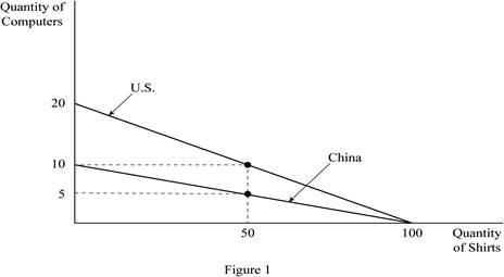
Figure 1 shows the production possibilities frontiers for the two countries; U.S. and China. In Figure 1, the horizontal axis measures the quantity of shirts produced by both the countries and the vertical axis measures the quantity of computers produced. If either worker of the two countries, that is an American or a Chinese worker devotes all his labor hours in producing shirts, each worker can produce 100 shirts in a year. Then, it is the vertical intercept of the PPF for both the American and the Chinese worker. If they devote all of their time to the production of computers, then the U.S. worker can produce 20 computers in a year, while the Chinese worker can produce only 10 computers per year. These are the horizontal intercepts of the PPF for the U.S. and the Chinese worker, respectively. Since the
Concept introduction:
Production possibility frontier (PPF): PPF is a curve depicting all maximum output possibilities for two goods, given a set of inputs consisting of resources and other factors.
Subpart (b):
Opportunity cost and price of the good.
Subpart (b):
Explanation of Solution
To determine the export pattern of shirts, the
Opportunity cost of shirts in the U.S. is calculated as,
Thus, the price of 1 shirt in the U.S. is 0.2 computers.
Opportunity cost of shirts in China is calculated as,
Thus, the price of 1 shirt in China is 0.1 computers.
Since China has a lower opportunity cost of shirts, China has a comparative advantage in its production. So, China will produce and export shirts to the U.S. in exchange for computers from the U.S. since the latter has a comparative advantage in the production of computers (5 shirts
The range of prices of shirts at which trade can occur is between 0.1 and 0.2 computers, per computer.
An example would be a price of 0.15 computers. Suppose China produced only shirts (100 shirts) and exported 50 shirts in exchange for 7.5
The United States is also benefited from this trade. Suppose American workers produced only computers (20 computers) and traded 7.5 of computers to China for 50 shirts. The U.S. would have 12.5 (20-7.5) computers and 50 shirts. Thus, the U.S. would be better off than before trade (10 computers and 50 shirts).
Concept introduction:
Production possibility frontier (PPF): PPF is a curve depicting all maximum output possibilities for two goods, given a set of inputs consisting of resources and other factors.
Opportunity cost: Opportunity cost is the cost of foregone alternative, that is, loss of an alternative when another alternative is chosen.
Comparative advantage: It refers to the ability to produce a good at a lower opportunity cost than another producer.
Subpart (c):
Opportunity cost and price of the good.
Subpart (c):
Explanation of Solution
For the calculation of price, the calculation of opportunity cost is required.
Opportunity cost of a computer in the U.S. is calculated as,
Thus, the price of 1 computer in the U.S. is 5 shirts.
Opportunity cost of a computer in China is calculated as,
Thus, the price of 1 computer in China is 10 shirts.
The range of prices of computers at which trade can occur is between 5 and 10 shirts per computer. This is because, at a price lower than 5 shirts, the U.S. will choose to produce its own shirts and will be unwilling to export computers, as the opportunity cost of a shirt for the U.S. is 0.2
Concept introduction:
Production possibility frontier (PPF): PPF is a curve depicting all maximum output possibilities for two goods, given a set of inputs consisting of resources and other factors.
Opportunity cost: Opportunity cost is the cost of foregone alternative, that is, loss of an alternative when another alternative is chosen.
Comparative advantage: It refers to the ability to produce a good at a lower opportunity cost than another producer.
Subpart (d):
Gains from the trade.
Subpart (d):
Explanation of Solution
Concept introduction:
Specialization: Specialization refers to allocate the work according to their efficiency. If an individual, company or country has produced a good at lower opportunity cost, then that particular individual, company or country should produce those goods.
Trade: The trade refers to the exchange of capital, goods, and services across different countries.
Want to see more full solutions like this?

- Answerarrow_forwardM” method Given the following model, solve by the method of “M”. (see image)arrow_forwardAs indicated in the attached image, U.S. earnings for high- and low-skill workers as measured by educational attainment began diverging in the 1980s. The remaining questions in this problem set use the model for the labor market developed in class to walk through potential explanations for this trend. 1. Assume that there are just two types of workers, low- and high-skill. As a result, there are two labor markets: supply and demand for low-skill workers and supply and demand for high-skill workers. Using two carefully drawn labor-market figures, show that an increase in the demand for high skill workers can explain an increase in the relative wage of high-skill workers. 2. Using the same assumptions as in the previous question, use two carefully drawn labor-market figures to show that an increase in the supply of low-skill workers can explain an increase in the relative wage of high-skill workers.arrow_forward
- Published in 1980, the book Free to Choose discusses how economists Milton Friedman and Rose Friedman proposed a one-sided view of the benefits of a voucher system. However, there are other economists who disagree about the potential effects of a voucher system.arrow_forwardThe following diagram illustrates the demand and marginal revenue curves facing a monopoly in an industry with no economies or diseconomies of scale. In the short and long run, MC = ATC. a. Calculate the values of profit, consumer surplus, and deadweight loss, and illustrate these on the graph. b. Repeat the calculations in part a, but now assume the monopoly is able to practice perfect price discrimination.arrow_forwardThe projects under the 'Build, Build, Build' program: how these projects improve connectivity and ease of doing business in the Philippines?arrow_forward
 Exploring EconomicsEconomicsISBN:9781544336329Author:Robert L. SextonPublisher:SAGE Publications, Inc
 Economics (MindTap Course List)EconomicsISBN:9781337617383Author:Roger A. ArnoldPublisher:Cengage Learning

 Economics Today and Tomorrow, Student EditionEconomicsISBN:9780078747663Author:McGraw-HillPublisher:Glencoe/McGraw-Hill School Pub Co
 Principles of Economics 2eEconomicsISBN:9781947172364Author:Steven A. Greenlaw; David ShapiroPublisher:OpenStax