Concept explainers
Videos
a.
Find the
a.
Answer to Problem 68SE
The median household income for 2013 is $52,100.
Explanation of Solution
Calculation:
The data represent the sample of 14 household incomes for 2013. It is also known that the median annual household income for 2007 was $55,500.
The variable “household income” is stored in the column “C1” in the MINITAB worksheet.
Median:
Software Procedure:
Step-by-step procedure to obtain the median using MINITAB software:
- Choose Stat > Basic Statistics > Display
Descriptive Statistics . - In Variables enter the columns C1.
- In Statistics select median.
- Click OK.
The output obtained using MINITAB software is given below:
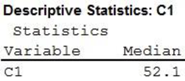
Thus, the median household income for 2013 is $52,100.
b.
Find the percentage change in the median household income from 2007 to 2013.
b.
Answer to Problem 68SE
The percentage change in the median household income from 2007 to 2013 is –6.1%.
Explanation of Solution
Calculation:
The median household income in 2007 is $55,500 (55.5). From Part (a), it can be seen that the median household income in 2013 is $52,100.
The percentage change in the median household income from 2007 to 2013 can be obtained as follows:
Thus, the percentage change in the median household income from 2007 to 2013 is –6.1%.
Therefore, there is 6.1% decrease in the median household income from 2007 to 2013.
c.
Find the first and third
c.
Answer to Problem 68SE
The first and third quartiles are $50,750 and $52,600, respectively.
Explanation of Solution
Calculation:
First quartile and Third quartile:
Software Procedure:
Step-by-step procedure to obtain the first and third quartiles using MINITAB software:
- Choose Stat > Basic Statistics >Display Descriptive Statistics.
- Click OK.
- In Variables, enter the column of C1.
- In Statistics select First quartile and Third quartile.
- Click OK.
The output obtained using MINITAB software is given below:
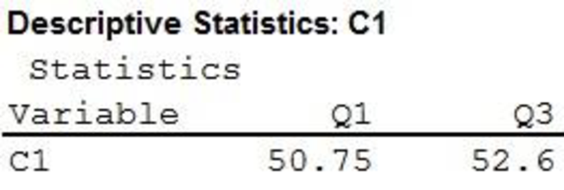
Therefore, the first and third quartiles are $50,750 and $52,600, respectively.
d.
Find the
d.
Answer to Problem 68SE
The five-number summary is as follows:
- Minimum: $46,500,
- First quartile: $50,750,
- Median: $52,100,
- Third quartile: $52,600,
- Maximum: $64,500.
Explanation of Solution
Calculation:
Five-number summary: Minimum, Q1, median, Q3, and maximum.
Five-number summary:
Software Procedure:
Step-by-step procedure to obtain the five-number summary using MINITAB software:
- Choose Stat > Basic Statistics >Display Descriptive Statistics.
- Click OK.
- In Variables, enter the column of C1.
- In Statistics, select Minimum, First quartile, Median, Third quartile and Maximum.
- Click OK.
The output obtained using MINITAB software is given below:
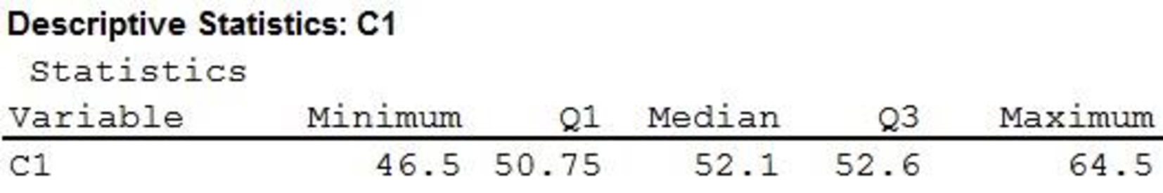
Thus, the five-number summary for data has been obtained.
e.
Identify the outliers using the z-score approach.
Check whether the approach that uses the values of the first and third quartiles and the
e.
Answer to Problem 68SE
The outlier obtained using the z-score approach is $64,500.
No, the approach that uses the values of the first and third quartiles and the interquartile
Explanation of Solution
Calculation:
The z-score:
where
Mean and Standard deviation:
Software Procedure:
Step-by-step procedure to obtain the mean and standard deviation using MINITAB software:
- Choose Stat > Basic Statistics > Display Descriptive Statistics.
- Click OK.
- In Variables, enter the column of C1.
- In Statistics select Mean and Standard deviation.
- Click OK.
The output obtained using MINITAB software is given below:
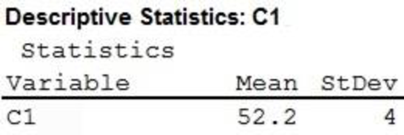
From the MINITAB output, it is clear that the mean and standard deviation are 52.2 and 4, respectively.
The z-score corresponding to 49.4 can be obtained as follows:
Substitute
Thus, the z-score corresponding to 49.4 is –0.70.
Similarly, the z-scores corresponding to other values can be obtained as follows:
| Values | z-score |
| 46.5 | –1.42 |
| 48.7 | –0.87 |
| 49.4 | –0.70 |
| 51.2 | –0.25 |
| 51.3 | –0.22 |
| 51.6 | –0.15 |
| 52.1 | –0.02 |
| 52.1 | –0.02 |
| 52.2 | 0.00 |
| 52.4 | 0.05 |
| 52.5 | 0.07 |
| 52.9 | 0.17 |
| 53.4 | 0.30 |
| 64.5 | 3.07 |
Outlier detection using the 3 standard deviation distance criterion:
An observation is considered as a potential outlier if the absolute value of the z-score of the observation is greater than 3, that is, if the observation lies more than 3 standard deviations away (above or below) from the mean value.
From the table, it can be seen that the z-score corresponding to 64.5 is greater than 3. Thus, the observation of 64.5 is considered to be an outlier.
Interquartile range (IQR):
- The outliers in the data set can be obtained as shown below:
By substituting the corresponding values, we obtain the following results:
A value in the dataset is said to be an outlier if it falls outside the interval from 47.98 to 55.375. In general, the data values less than 47.98 or greater than 55.375 are considered as the outliers.
The first observation (46.5) is less than 47.98, and the observation (64.5) is greater than 55.375. Hence, there are two outliers, $49,400 and $64,500.
Thus, the results obtained in two approaches are not the same.
Want to see more full solutions like this?
Chapter 3 Solutions
Essentials of Statistics for Business and Economics (with XLSTAT Printed Access Card)


- Questions An insurance company's cumulative incurred claims for the last 5 accident years are given in the following table: Development Year Accident Year 0 2018 1 2 3 4 245 267 274 289 292 2019 255 276 288 294 2020 265 283 292 2021 263 278 2022 271 It can be assumed that claims are fully run off after 4 years. The premiums received for each year are: Accident Year Premium 2018 306 2019 312 2020 318 2021 326 2022 330 You do not need to make any allowance for inflation. 1. (a) Calculate the reserve at the end of 2022 using the basic chain ladder method. (b) Calculate the reserve at the end of 2022 using the Bornhuetter-Ferguson method. 2. Comment on the differences in the reserves produced by the methods in Part 1.arrow_forwardYou are provided with data that includes all 50 states of the United States. Your task is to draw a sample of: o 20 States using Random Sampling (2 points: 1 for random number generation; 1 for random sample) o 10 States using Systematic Sampling (4 points: 1 for random numbers generation; 1 for random sample different from the previous answer; 1 for correct K value calculation table; 1 for correct sample drawn by using systematic sampling) (For systematic sampling, do not use the original data directly. Instead, first randomize the data, and then use the randomized dataset to draw your sample. Furthermore, do not use the random list previously generated, instead, generate a new random sample for this part. For more details, please see the snapshot provided at the end.) Upload a Microsoft Excel file with two separate sheets. One sheet provides random sampling while the other provides systematic sampling. Excel snapshots that can help you in organizing columns are provided on the next…arrow_forwardThe population mean and standard deviation are given below. Find the required probability and determine whether the given sample mean would be considered unusual. For a sample of n = 65, find the probability of a sample mean being greater than 225 if μ = 224 and σ = 3.5. For a sample of n = 65, the probability of a sample mean being greater than 225 if μ=224 and σ = 3.5 is 0.0102 (Round to four decimal places as needed.)arrow_forward
- ***Please do not just simply copy and paste the other solution for this problem posted on bartleby as that solution does not have all of the parts completed for this problem. Please answer this I will leave a like on the problem. The data needed to answer this question is given in the following link (file is on view only so if you would like to make a copy to make it easier for yourself feel free to do so) https://docs.google.com/spreadsheets/d/1aV5rsxdNjHnkeTkm5VqHzBXZgW-Ptbs3vqwk0SYiQPo/edit?usp=sharingarrow_forwardThe data needed to answer this question is given in the following link (file is on view only so if you would like to make a copy to make it easier for yourself feel free to do so) https://docs.google.com/spreadsheets/d/1aV5rsxdNjHnkeTkm5VqHzBXZgW-Ptbs3vqwk0SYiQPo/edit?usp=sharingarrow_forwardThe following relates to Problems 4 and 5. Christchurch, New Zealand experienced a major earthquake on February 22, 2011. It destroyed 100,000 homes. Data were collected on a sample of 300 damaged homes. These data are saved in the file called CIEG315 Homework 4 data.xlsx, which is available on Canvas under Files. A subset of the data is shown in the accompanying table. Two of the variables are qualitative in nature: Wall construction and roof construction. Two of the variables are quantitative: (1) Peak ground acceleration (PGA), a measure of the intensity of ground shaking that the home experienced in the earthquake (in units of acceleration of gravity, g); (2) Damage, which indicates the amount of damage experienced in the earthquake in New Zealand dollars; and (3) Building value, the pre-earthquake value of the home in New Zealand dollars. PGA (g) Damage (NZ$) Building Value (NZ$) Wall Construction Roof Construction Property ID 1 0.645 2 0.101 141,416 2,826 253,000 B 305,000 B T 3…arrow_forward
- Rose Par posted Apr 5, 2025 9:01 PM Subscribe To: Store Owner From: Rose Par, Manager Subject: Decision About Selling Custom Flower Bouquets Date: April 5, 2025 Our shop, which prides itself on selling handmade gifts and cultural items, has recently received inquiries from customers about the availability of fresh flower bouquets for special occasions. This has prompted me to consider whether we should introduce custom flower bouquets in our shop. We need to decide whether to start offering this new product. There are three options: provide a complete selection of custom bouquets for events like birthdays and anniversaries, start small with just a few ready-made flower arrangements, or do not add flowers. There are also three possible outcomes. First, we might see high demand, and the bouquets could sell quickly. Second, we might have medium demand, with a few sold each week. Third, there might be low demand, and the flowers may not sell well, possibly going to waste. These outcomes…arrow_forwardConsider the state space model X₁ = §Xt−1 + Wt, Yt = AX+Vt, where Xt Є R4 and Y E R². Suppose we know the covariance matrices for Wt and Vt. How many unknown parameters are there in the model?arrow_forwardBusiness Discussarrow_forward
- You want to obtain a sample to estimate the proportion of a population that possess a particular genetic marker. Based on previous evidence, you believe approximately p∗=11% of the population have the genetic marker. You would like to be 90% confident that your estimate is within 0.5% of the true population proportion. How large of a sample size is required?n = (Wrong: 10,603) Do not round mid-calculation. However, you may use a critical value accurate to three decimal places.arrow_forward2. [20] Let {X1,..., Xn} be a random sample from Ber(p), where p = (0, 1). Consider two estimators of the parameter p: 1 p=X_and_p= n+2 (x+1). For each of p and p, find the bias and MSE.arrow_forward1. [20] The joint PDF of RVs X and Y is given by xe-(z+y), r>0, y > 0, fx,y(x, y) = 0, otherwise. (a) Find P(0X≤1, 1arrow_forwardarrow_back_iosSEE MORE QUESTIONSarrow_forward_ios
 Big Ideas Math A Bridge To Success Algebra 1: Stu...AlgebraISBN:9781680331141Author:HOUGHTON MIFFLIN HARCOURTPublisher:Houghton Mifflin Harcourt
 Glencoe Algebra 1, Student Edition, 9780079039897...AlgebraISBN:9780079039897Author:CarterPublisher:McGraw Hill
 Holt Mcdougal Larson Pre-algebra: Student Edition...AlgebraISBN:9780547587776Author:HOLT MCDOUGALPublisher:HOLT MCDOUGAL