Principles Of Economics 2e
2nd Edition
ISBN: 9781680920864
Author: Timothy Taylor, Steven A. Greenlaw, David Shapiro
Publisher: MCGRAW-HILL HIGHER EDUCATION
expand_more
expand_more
format_list_bulleted
Textbook Question
Chapter 3, Problem 36CTQ
Review Figure 3.4. Suppose the government decided that, since gasoline is a necessity, its
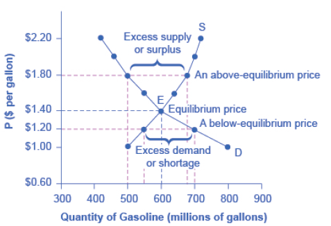
Figure 3.4
Expert Solution & Answer

Trending nowThis is a popular solution!

Students have asked these similar questions
At the 8:10 café, there are equal numbers of two types of customers with the following values. The café owner cannot distinguish between the two types of students because many students without early classes arrive early anyway (that is she cannot price discriminate).
Students with early classes
Students without early classes
Coffee
70
60
Banana
50
100
The MC of coffee is 10. The MC of a banana is 40. Is bundling more profitable than selling separately? HINT: if you sell the bundle, can you make more by offering coffee separately?
If so, what price should be charged for the bundle? (Show calculations)
Your marketing department has identified the following customer demographics in the following table. Construct a demand curve and determine the profit maximizing price as well as the expected profit if MC=$1. The number of customers in the target population is 10,000.
Use the following demand data:
Group
Value
Frequency
Baby boomers
$5
20%
Generation X
$4
10%
Generation Y
$3
10%
`Tweeners
$2
10%
Seniors
$2
10%
Others
$0
40%
Your marketing department has identified the following customer demographics in the following table. Construct a demand curve and determine the profit maximizing price as well as the expected profit if MC=$1. The number of customers in the target population is 10,000.
Group
Value
Frequency
Baby boomers
$5
20%
Generation X
$4
10%
Generation Y
$3
10%
`Tweeners
$2
10%
Seniors
$2
10%
Others
$0
40%
ur marketing department has identified the following customer demographics in the following table. Construct a demand curve and determine the profit maximizing price as well as the expected profit if MC=$1. The number of customers in the target population is 10,000.
Chapter 3 Solutions
Principles Of Economics 2e
Ch. 3 - Review Figure 3.4. Suppose the price of gasoline...Ch. 3 - Why do economists use the ceteris paribus...Ch. 3 - In an analysis of the market for paint, an...Ch. 3 - Many changes are affecting the market for oil....Ch. 3 - Lets think about the market for air travel. From...Ch. 3 - A tariff is a tax on imported goods. Suppose the...Ch. 3 - What is the effect of a price ceiling on the...Ch. 3 - Does a price ceiling change the equilibrium price?Ch. 3 - What would be the impact of imposing a price flour...Ch. 3 - Does a price ceiling increase the decrease the...
Ch. 3 - If a price floor benefits producers, why does a...Ch. 3 - What determines the level of prices in a market?Ch. 3 - What does a downward-sloping demand curve mean...Ch. 3 - Will demand curves have the same exact shape in...Ch. 3 - Will supply curves have the same shape in all...Ch. 3 - What is the relationship between quantity Demanded...Ch. 3 - How can you locate the equilibrium point on a...Ch. 3 - If the price is above line equilibrium level,...Ch. 3 - When the price is above the equilibrium, explain...Ch. 3 - What is the difference between the demand and the...Ch. 3 - What is the difference between the supply and the...Ch. 3 - When analyzing a market, how do economists deal...Ch. 3 - Name some factors that can cause a shift in line...Ch. 3 - Name some farm that can cause a shift in the...Ch. 3 - How does one analyze a market where both demand...Ch. 3 - What causes a movement along the demand curve?...Ch. 3 - Does a price ceiling attempt to make a price...Ch. 3 - How does a price ceiling set below the equilibrium...Ch. 3 - Does a price floor attempt to make a price higher...Ch. 3 - How does a price floor 521 above the equilibrium...Ch. 3 - What is consumer surplus? How is it illustrated on...Ch. 3 - What is producer surplus? How is it illustrated on...Ch. 3 - What is total surplus? How is it illustrated on a...Ch. 3 - What is the relationship between total surplus and...Ch. 3 - What is deadweight loss?Ch. 3 - Review Figure 3.4. Suppose the government decided...Ch. 3 - Explain why the following statement is false: In...Ch. 3 - Explain why the following statement is false: In...Ch. 3 - Consider the demand for hamburgers. If the price...Ch. 3 - How do you suppose the demographics of an aging...Ch. 3 - We know that a change in the price of a product...Ch. 3 - Suppose there is a soda tax to curb obesity. What...Ch. 3 - Use the four-step process to analyze the impact of...Ch. 3 - Use the four-step process to analyze the impact of...Ch. 3 - Suppose both of these events took place at the...Ch. 3 - Must government policy decisions have winners and...Ch. 3 - Agricultural price supports result in governments...Ch. 3 - Can you propose a policy that meld induce the...Ch. 3 - What term would an economist use to describe what...Ch. 3 - Explain why voluntary Martians improve social...Ch. 3 - Why would a free market mar operate at a quantity...Ch. 3 - Review Figure 3.4 again. Suppose the price of...Ch. 3 - Table 3.8 shows information on the demand and...Ch. 3 - The computer market in recent years has seen many...Ch. 3 - Table 3.9 illustrates the markets demand and...Ch. 3 - Table 3.10 shows the supply and demand for movie...Ch. 3 - A low-income county decides to set a price ceiling...
Additional Business Textbook Solutions
Find more solutions based on key concepts
Create an Excel spreadsheet on your own that can make combination forecasts for Problem 18. Create a combinatio...
Operations Management: Processes and Supply Chains (12th Edition) (What's New in Operations Management)
A company has the opportunity to take over a redevelopment project in an industrial area of a city. No immediat...
Engineering Economy (17th Edition)
Small Business Analysis Purpose: To help you understand the importance of cash flows in the operation of a smal...
Financial Accounting, Student Value Edition (5th Edition)
E2-13 Identifying increases and decreases in accounts and normal balances
Learning Objective 2
Insert the mis...
Horngren's Accounting (12th Edition)
To calculate the current WACC. Introduction: The weighted average cost of capital is defined as the expected av...
Gitman: Principl Manageri Finance_15 (15th Edition) (What's New in Finance)
Knowledge Booster

Similar questions
- Test Preparation QUESTION 2 [20] 2.1 Body Mass Index (BMI) is a summary measure of relative health. It is calculated by dividing an individual's weight (in kilograms) by the square of their height (in meters). A small sample was drawn from the population of UWC students to determine the effect of exercise on BMI score. Given the following table, find the constant and slope parameters of the sample regression function of BMI = f(Weekly exercise hours). Interpret the two estimated parameter values. X (Weekly exercise hours) Y (Body-Mass index) QUESTION 3 2 4 6 8 10 12 41 38 33 27 23 19 Derek investigates the relationship between the days (per year) absent from work (ABSENT) and the number of years taken for the worker to be promoted (PROMOTION). He interviewed a sample of 22 employees in Cape Town to obtain information on ABSENT (X) and PROMOTION (Y), and derived the following: ΣΧ ΣΥ 341 ΣΧΥ 176 ΣΧ 1187 1012 3.1 By using the OLS method, prove that the constant and slope parameters of the…arrow_forwardQUESTION 2 2.1 [30] Mariana, a researcher at the World Health Organisation (WHO), collects information on weekly study hours (HOURS) and blood pressure level when writing a test (BLOOD) from a sample of university students across the country, before running the regression BLOOD = f(STUDY). She collects data from 5 students as listed below: X (STUDY) 2 Y (BLOOD) 4 6 8 10 141 138 133 127 123 2.1.1 By using the OLS method and the information above derive the values for parameters B1 and B2. 2.1.2 Derive the RSS (sum of squares for the residuals). 2.1.3 Hence, calculate ô 2.2 2.3 (6) (3) Further, she replicates her study and collects data from 122 students from a rival university. She derives the residuals followed by computing skewness (S) equals -1.25 and kurtosis (K) equals 8.25 for the rival university data. Conduct the Jacque-Bera test of normality at a = 0.05. (5) Upon tasked with deriving estimates of ẞ1, B2, 82 and the standard errors (SE) of ẞ1 and B₂ for the replicated data.…arrow_forwardIf you were put in charge of ensuring that the mining industry in canada becomes more sustainable over the course of the next decade (2025-2035), how would you approach this? Come up with (at least) one resolution for each of the 4 major types of conflict: social, environmental, economic, and politicalarrow_forward
- How is the mining industry related to other Canadian labour industries? Choose one other industry, (I chose Forestry)and describe how it is related to the mining industry. How do the two industries work together? Do they ever conflict, or do they work well together?arrow_forwardWhat is the primary, secondary, tertiary, and quaternary levels of mining in Canada For each level, describe what types of careers are the most common, and describe what stage your industry’s main resource is in during that stagearrow_forwardHow does the mining industry in canada contribute to the Canadian economy? Describe why your industry is so important to the Canadian economy What would happen if your industry disappeared, or suffered significant layoffs?arrow_forward
- What is already being done to make mining in canada more sustainable? What efforts are being made in order to make mining more sustainable?arrow_forwardWhat are the environmental challenges the canadian mining industry face? Discuss current challenges that mining faces with regard to the environmentarrow_forwardWhat sustainability efforts have been put forth in the mining industry in canada Are your industry’s resources renewable or non-renewable? How do you know? Describe your industry’s reclamation processarrow_forward
- How does oligopolies practice non-price competition in South Africa?arrow_forwardWhat are the advantages and disadvantages of oligopolies on the consumers, businesses and the economy as a whole?arrow_forward1. After the reopening of borders with mainland China following the COVID-19 lockdown, residents living near the border now have the option to shop for food on either side. In Hong Kong, the cost of food is at its listed price, while across the border in mainland China, the price is only half that of Hong Kong's. A recent report indicates a decline in food sales in Hong Kong post-reopening. ** Diagrams need not be to scale; Focus on accurately representing the relevant concepts and relationships rather than the exact proportions. (a) Using a diagram, explain why Hong Kong's food sales might have dropped after the border reopening. Assume that consumers are indifferent between purchasing food in Hong Kong or mainland China, and therefore, their indifference curves have a slope of one like below. Additionally, consider that there are no transport costs and the daily food budget for consumers is identical whether they shop in Hong Kong or mainland China. I 3. 14 (b) In response to the…arrow_forward
arrow_back_ios
SEE MORE QUESTIONS
arrow_forward_ios
Recommended textbooks for you

 Microeconomics: Principles & PolicyEconomicsISBN:9781337794992Author:William J. Baumol, Alan S. Blinder, John L. SolowPublisher:Cengage Learning
 Managerial Economics: A Problem Solving ApproachEconomicsISBN:9781337106665Author:Luke M. Froeb, Brian T. McCann, Michael R. Ward, Mike ShorPublisher:Cengage Learning
 Economics (MindTap Course List)EconomicsISBN:9781337617383Author:Roger A. ArnoldPublisher:Cengage Learning

Microeconomics: Principles & Policy
Economics
ISBN:9781337794992
Author:William J. Baumol, Alan S. Blinder, John L. Solow
Publisher:Cengage Learning
Managerial Economics: A Problem Solving Approach
Economics
ISBN:9781337106665
Author:Luke M. Froeb, Brian T. McCann, Michael R. Ward, Mike Shor
Publisher:Cengage Learning
Economics (MindTap Course List)
Economics
ISBN:9781337617383
Author:Roger A. Arnold
Publisher:Cengage Learning