Chapter 3, Problem 3.1P

A

To determine

To find:The number of shoes and jeans that the individual buys, if jeans cost $20 and shoes cost $20.

Answer to Problem 3.1P

At the given constraints and the data, the individual will be able to buy 5 pairs of both jeans and shoes.

Explanation of Solution

First, let us assume that the income of the individual is represented by, I = $200. While the jeans is represented by J, P_J for price of Jeans; shoes is represented by S, P_S for price of shoes.

So, the equation denoting the budget constraint of the individual can be defined as follows:

  $\begin{array}{l}{P}_J.J+P_S.S=I\\ P_J.J+P_S.S=\$200\end{array}$

Since, the individual buys the two goods in the same number,

J=S

Now,

P_J=$20, and P_S=$20; and J=S

Now, by substituting the price of two goods in the above equation,

  $\begin{array}{l}\$20J+\$20S=\$200\\ \$20J+\$20J=\$200\\ \$40J=\$200\\ J=5\end{array}$

Thus, we can see that the individual will be able to buy only 5 units of both jeans and shoes.

Economics Concept Introduction

The budget constraint details the combinations of goods and services that an individual may acquire at the possible prices, within the income level of the individual.

B

To determine

To find:The number of shoes and jeans that the individual will buy after increase in price of jeans to $30

Answer to Problem 3.1P

The individual, according to the given data, will be able to purchase 4 units of both shoes and jeans.

Explanation of Solution

Now, the price of Jeans is, P_J=$30, and the price of Shoes is, P_J=$20.

Substituting the prices into equation,

  $\begin{array}{l}\$30J+\$20S=200\\ \$50J=\$200\\ J=4\end{array}$

Thus, at the given constraint, the individual will be able to buy 4 units of both jeans and shoes.

Economics Concept Introduction

The budget constraint details the combinations of goods and services that an individual may acquire at the possible prices, within the income level of the individual.

C

To determine

To plot:The budget constraints from parts A and B on a graph.

Answer to Problem 3.1P

We can notice on the graph that the indifference curves have transformed into L-shape, showing that the jeans and shoes are bought in an equal proportion meaning that they are perfect complements.

Explanation of Solution

  

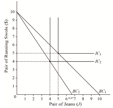
Through plotting the budget constraints and indifference curves on the graph, it is that the BC₁ and IC₁ represent the budget constraint and the indifference curve, representing the price of Jeans, P_J=$20, and the price of shoes, P_S=$20, respectively.

Similarly, the BC₂ and IC₂represent the budget constraint and the indifference curve, representing the price of Jeans, P_J=$30, and the price of shoes, P_S=$20, respectively.

It is noticed on the graph that the indifference curves have transformed into L-shape, showing that the jeans and shoes are bought in an equal proportion. Meaning that they are perfect complements.

Economics Concept Introduction

The budget constraint details the combinations of goods and services that an individual may acquire at the possible prices, within the income level of the individual.

D

To determine

To find: the change that can be attributed by the change in utility levels among the parts A and B

Answer to Problem 3.1P

Since, the individual is purchasing the jeans and shoes in a fixed proportion, the changes in utility levels, represented by IC₁ and IC₂, can be attributed completely to the income effect.

Explanation of Solution

By looking at the graph, it can be noticed that the utility levels IC₁ and IC₂ are perpendicular, meaning that the purchases of shoes and jeans are made in a fixed proportion.

Hence, the changes in utility levels are attributed entirely to the income effect.

Economics Concept Introduction

Introduction: The budget constraint details the combinations of goods and services that an individual may acquire at the possible prices, within the income level of the individual.

E

To determine

To Find:the number of jeans that the individual will purchase at different prices of$30, $20, $10, and $5.

Answer to Problem 3.1P

At a price of $30, the demanded pair of jeans are 4;

at $20, 5 pairs;

at $10, 6 pairs;

at $5, 8 pairs are demanded.

Explanation of Solution

Jeans priced at $30, and Shoes priced at $20, the pair of jeans demanded are as follows:

  $\begin{array}{l}\$30J+\$20J=\$200\\ \$50J=\$200\\ J=4\end{array}$

Jeans priced at $20, and Shoes priced at $20, the pair of jeans demanded are as follows:

  $\begin{array}{l}\$20J+\$20J=\$200\\ \$40J=\$200\\ J=5\end{array}$

Jeans priced at $10, and Shoes priced at $20, the pair of jeans demanded are as follows:

  $\begin{array}{l}\$10J+\$20J=\$200\\ \$30J=\$200\\ J=6\end{array}$

Jeans priced at $5, and Shoes priced at $20, the pair of jeans demanded are as follows:

  $\begin{array}{l}\$5J+\$20J=\$200\\ \$25J=\$200\\ J=8\end{array}$

Economics Concept Introduction

Introduction: The budget constraint details the combinations of goods and services that an individual may acquire at the possible prices, within the income level of the individual.

F

To determine

To plot: using the demand pattern derived from part E, the demand curve on the graph.

Answer to Problem 3.1P

The demand curve is sloping downward.

Explanation of Solution

  

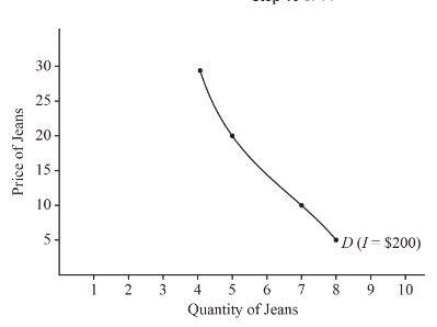
By looking at the demand curve plotted on the graph, we can notice that with every increase in the price of Jeans, the demand has increased.

Economics Concept Introduction

Introduction: The budget constraint details the combinations of goods and services that an individual may acquire at the possible prices, within the income level of the individual.

G

To determine

To plot:the demand curve on a graphsupposing that the income of the individual rises to $300, also to derive the demand for jeans at each price level.

Answer to Problem 3.1P

The demand curve has extended with an increase in the income level of the individual.

Explanation of Solution

By substituting the new income level in the derived equation, itis seen that the following demand pattern is observed at every price change:

Price of Jeans	Demand for Jeans
$30	6
$20	7
$10	10
$5	12

  

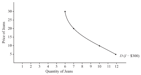
Through plotting this new demand curve with an increased income level, it is noticed that the demand curve has extended with an increase in the income level of the individual.

Economics Concept Introduction

Introduction: The budget constraint details the combinations of goods and services that an individual may acquire at the possible prices, within the income level of the individual.

H

To determine

To find:supposing that the price of the shoes rises to $30 per pair,the effect on demand curves drawn in parts B and C.

Answer to Problem 3.1P

The demand curve will shift to the left showing a decline in the demand for jeans at the given price levels.

Explanation of Solution

As stated, the demand for jeans and shoes is in a fixed proportion. Hence, with an increase in the price of shoes, the demand for both jeans and shoes will show a decline. Thus, it is noticed that the demand curve will shift to left, representing a decline in the demand for jeans at the given price levels.

Economics Concept Introduction

Introduction: The budget constraint details the combinations of goods and services that an individual may acquire at the possible prices, within the income level of the individual.