
Concept explainers
(a)
(a)
Explanation of Solution
The given information:
Supply equation for ice cream is
Calculation:
Rearrange Equation (1) in terms of
The inverse demand equation is
Rearrange Equation (2) in terms of price derive the inverse supply equation.
The inverse supply equation is
The intersecting point of the demand and supply curve is the equilibrium point. Calculation of equilibrium price is shown below:
Equilibrium price is $5.
Substitute the price in the demand equation (Equation (1)) to calculate the equilibrium quantity.
Equilibrium quantity is 10 units (10 gallon of ice cream).
From the above information, the market for ice cream is shown below:
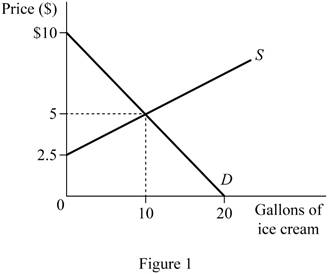
In Figure 1, the vertical axis measures the price of ice cream and the horizontal axis measures gallon of ice cream. The upward sloping curve is the supply curve and downward sloping curve is the demand curve of ice cream. The intersecting point of the demand and supply curve is the equilibrium point. Thus, the equilibrium price is $5 and quantity is 10 units.
(b)
New demand equation.
(b)
Explanation of Solution
The imposition of tax increases the price, when price increases, the demand for the goods will decrease, which shifts the demand curve leftward. The new demand curve is shown in below figure.
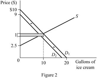
In Figure 2, the vertical axis measures the price of ice cream and the horizontal axis measures the gallon of ice cream. The upward sloping curve is the supply curve and downward sloping curve is the demand curve of ice cream. The demand curve shift inward by the imposition of tax by $1.
(c)
New price and quantity.
(c)
Explanation of Solution
The new demand equation can be written as follows:
The new demand equation is
The new equilibrium price can be calculated as follows:
The new price is $4.67.
Substitute the price in the demand equation (Equation (2)) to calculate the
New quantity is 8.68 units.
(d)
Burden of tax.
(d)
Explanation of Solution
After imposition of tax ($1), the buyer would pay $5.67
(e)
(e)
Explanation of Solution
To find out the consumer surplus, the choke price has to be calculated. The calculation of choke price is shown below:
Substitute the value of quantity as zero in Equation (1).
The demand choke price (maximum willing price) is $10.
Consumer surplus before tax imposition is calculated as follows:
Consumer surplus is $25.
Consumer surplus after tax imposition is calculated as follows:
To find out the consumer surplus after tax, the choke price has to be calculated. The calculation of choke price is shown below:
Substitute the value of quantity as zero in Equation (5).
The demand choke price (maximum willing price) is $9.
Consumer surplus after tax imposition is calculated as follows:
Consumer surplus is $18.79.
(f)
Producer surplus.
(f)
Explanation of Solution
To find out the producer surplus, the choke price has to be calculated. The calculation of choke price is shown below:
Substitute the value of quantity as zero in Equation (2).
The supply choke price (minimum acceptable price) is $2.5.
Producer surplus before tax imposition is calculated as follows:
Producer surplus is $12.50.
Producer surplus after tax imposition is calculated as follows”
Producer surplus is $9.42.
(g)
Total tax revenue.
(g)
Explanation of Solution
Total tax revenue can be calculated as follows:
Tax revenue is $8.68.
(h)
(h)
Explanation of Solution
Deadweight loss can be calculated as follows:
Deadweight loss is $0.66.
Want to see more full solutions like this?
Chapter 3 Solutions
EBK MICROECONOMICS


- How does the mining industry in canada contribute to the Canadian economy? Describe why your industry is so important to the Canadian economy What would happen if your industry disappeared, or suffered significant layoffs?arrow_forwardWhat is already being done to make mining in canada more sustainable? What efforts are being made in order to make mining more sustainable?arrow_forwardWhat are the environmental challenges the canadian mining industry face? Discuss current challenges that mining faces with regard to the environmentarrow_forward
- What sustainability efforts have been put forth in the mining industry in canada Are your industry’s resources renewable or non-renewable? How do you know? Describe your industry’s reclamation processarrow_forwardHow does oligopolies practice non-price competition in South Africa?arrow_forwardWhat are the advantages and disadvantages of oligopolies on the consumers, businesses and the economy as a whole?arrow_forward
- 1. After the reopening of borders with mainland China following the COVID-19 lockdown, residents living near the border now have the option to shop for food on either side. In Hong Kong, the cost of food is at its listed price, while across the border in mainland China, the price is only half that of Hong Kong's. A recent report indicates a decline in food sales in Hong Kong post-reopening. ** Diagrams need not be to scale; Focus on accurately representing the relevant concepts and relationships rather than the exact proportions. (a) Using a diagram, explain why Hong Kong's food sales might have dropped after the border reopening. Assume that consumers are indifferent between purchasing food in Hong Kong or mainland China, and therefore, their indifference curves have a slope of one like below. Additionally, consider that there are no transport costs and the daily food budget for consumers is identical whether they shop in Hong Kong or mainland China. I 3. 14 (b) In response to the…arrow_forward2. Health Food Company is a well-known global brand that specializes in healthy and organic food products. One of their main products is organic chicken, which they source from small farmers in the area. Health Food Company is the sole buyer of organic chicken in the market. (a) In the context of the organic chicken industry, what type of market structure is Health Food Company operating in? (b) Using a diagram, explain how the identified market structure affects the input pricing and output decisions of Health Food Company. Specifically, include the relevant curves and any key points such as the profit-maximizing price and quantity. () (c) How can encouraging small chicken farmers to form bargaining associations help improve their trade terms? Explain how this works by drawing on the graph in answer (b) to illustrate your answer.arrow_forward2. Suppose that a farmer has two ways to produce his crop. He can use a low-polluting technology with the marginal cost curve MCL or a high polluting technology with the marginal cost curve MCH. If the farmer uses the high-polluting technology, for each unit of quantity produced, one unit of pollution is also produced. Pollution causes pollution damages that are valued at $E per unit. The good produced can be sold in the market for $P per unit. P 1 MCH 0 Q₁ MCL Q2 E a. b. C. If there are no restrictions on the firm's choices, which technology will the farmer use and what quantity will he produce? Explain, referring to the area identified in the figure Given your response in part a, is it socially efficient for there to be no restriction on production? Explain, referring to the area identified in the figure If the government restricts production to Q1, what technology would the farmer choose? Would a socially efficient outcome be achieved? Explain, referring to the area identified in…arrow_forward
- I need help in seeing how these are the answers. If you could please write down your steps so I can see how it's done please.arrow_forwardSuppose that a random sample of 216 twenty-year-old men is selected from a population and that their heights and weights are recorded. A regression of weight on height yields Weight = (-107.3628) + 4.2552 x Height, R2 = 0.875, SER = 11.0160 (2.3220) (0.3348) where Weight is measured in pounds and Height is measured in inches. A man has a late growth spurt and grows 1.6200 inches over the course of a year. Construct a confidence interval of 90% for the person's weight gain. The 90% confidence interval for the person's weight gain is ( ☐ ☐) (in pounds). (Round your responses to two decimal places.)arrow_forwardSuppose that (Y, X) satisfy the assumptions specified here. A random sample of n = 498 is drawn and yields Ŷ= 6.47 + 5.66X, R2 = 0.83, SER = 5.3 (3.7) (3.4) Where the numbers in parentheses are the standard errors of the estimated coefficients B₁ = 6.47 and B₁ = 5.66 respectively. Suppose you wanted to test that B₁ is zero at the 5% level. That is, Ho: B₁ = 0 vs. H₁: B₁ #0 Report the t-statistic and p-value for this test. Definition The t-statistic is (Round your response to two decimal places) ☑ The Least Squares Assumptions Y=Bo+B₁X+u, i = 1,..., n, where 1. The error term u; has conditional mean zero given X;: E (u;|X;) = 0; 2. (Y;, X¡), i = 1,..., n, are independent and identically distributed (i.i.d.) draws from i their joint distribution; and 3. Large outliers are unlikely: X; and Y, have nonzero finite fourth moments.arrow_forward

 Principles of Economics (12th Edition)EconomicsISBN:9780134078779Author:Karl E. Case, Ray C. Fair, Sharon E. OsterPublisher:PEARSON
 Engineering Economy (17th Edition)EconomicsISBN:9780134870069Author:William G. Sullivan, Elin M. Wicks, C. Patrick KoellingPublisher:PEARSON
 Principles of Economics (MindTap Course List)EconomicsISBN:9781305585126Author:N. Gregory MankiwPublisher:Cengage Learning
 Managerial Economics: A Problem Solving ApproachEconomicsISBN:9781337106665Author:Luke M. Froeb, Brian T. McCann, Michael R. Ward, Mike ShorPublisher:Cengage Learning
 Managerial Economics & Business Strategy (Mcgraw-...EconomicsISBN:9781259290619Author:Michael Baye, Jeff PrincePublisher:McGraw-Hill Education