
Concept explainers
Videos
(a)
Section 1:
To find: The 20 simple random samples of size 5 and record the number of instate students in each sample.
(a)
Section 1:
Answer to Problem 14E
Solution: The partial output of 20 simple random samples is shown below:
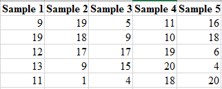
The number of instate players obtained in each set of samples is shown in the below table.
| Samples | Number of instate players | Samples | Number of instate players |
| Sample 1 | 2 | Sample 11 | 4 |
| Sample 2 | 1 | Sample 12 | 1 |
| Sample 3 | 2 | Sample 13 | 3 |
| Sample 4 | 2 | Sample 14 | 0 |
| Sample 5 | 1 | Sample 15 | 2 |
| Sample 6 | 0 | Sample 16 | 0 |
| Sample 7 | 3 | Sample 17 | 3 |
| Sample 8 | 3 | Sample 18 | 2 |
| Sample 9 | 1 | Sample 19 | 3 |
| Sample 10 | 4 | Sample 20 | 3 |
Explanation of Solution
Calculation:
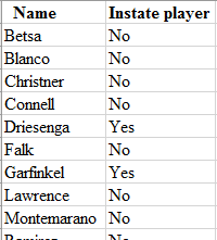
Step 1: In the Excel spreadsheet, write the name of the students and whether they are instate players or not. The snapshot is shown below:
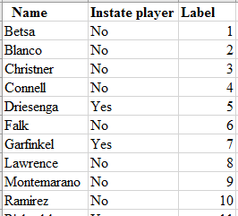
Step 2: Label each of the students using the numbers
Step 3: Use the formula

To find the number of instate players in each sample, the label of each instate players are matched with the obtained random number of each set of sample and calculate the number of instate players. The number of instate players obtained in each set of samples are shown in the below table.
| Samples | Number of instate players | Samples | Number of instate players |
| Sample 1 | 2 | Sample 11 | 4 |
| Sample 2 | 1 | Sample 12 | 1 |
| Sample 3 | 2 | Sample 13 | 3 |
| Sample 4 | 2 | Sample 14 | 0 |
| Sample 5 | 1 | Sample 15 | 2 |
| Sample 6 | 0 | Sample 16 | 0 |
| Sample 7 | 3 | Sample 17 | 3 |
| Sample 8 | 3 | Sample 18 | 2 |
| Sample 9 | 1 | Sample 19 | 3 |
| Sample 10 | 4 | Sample 20 | 3 |
Section 2:
To graph: The histogram for the number of instate players in each set of sample.
Section 2:
Answer to Problem 14E
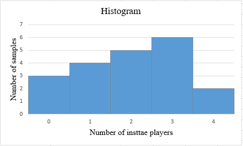
Solution: The obtained histogram is obtained as:
Explanation of Solution
Graph:
To obtain the histogram for the obtained result in previous part, Excel is used. The below steps are followed to obtained the required histogram.
Step 1: The number of instate players varies from 0 to 4. The number of samples are calculated corresponding to each number of instate players. The number of samples with same number of instate players are clustered. The snapshot of the obtained table is shown below:
| Number of instate players members | Number of samples |
| 0 | 3 |
| 1 | 4 |
| 2 | 5 |
| 3 | 6 |
| 4 | 2 |
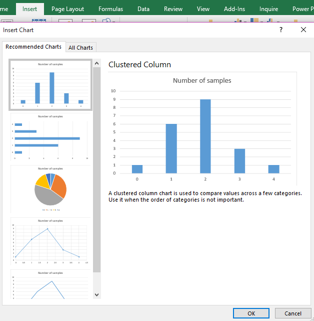
Step 2: Select the data set and go to insert and select the option of cluster column under the Recommended Charts. The screenshot is shown below:
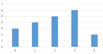
Step 3: Click on OK. The diagram is obtained as:
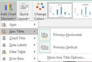
Step 4: Click on the chart area and select the option of “Primary Horizontal” and “Primary Vertical” axis under the “Add Chart Element” to add the axis title. The screenshot is shown below:
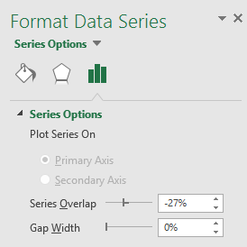
Step 5: Click on the bars of the diagrams and reduce the gap width to zero under the “Format Data Series” tab. The screenshot is shown below:
The obtained histogram is:

Section 3:
To find: The average number of instate players in 20 samples.
Section 3:
Answer to Problem 14E
Solution: The average number of instate players is 2.
Explanation of Solution
Explanation
Calculation:
The average number of instate players can be obtained by using the formula:
Hence, the average number of instate players is calculated as:
(b)
To explain: Whether the college should be doubtful about the discrimination if any of the five scholarships does not received by instate players.
(b)
Answer to Problem 14E
Solution: The college should suspect the discrimination if any of the five scholarships does not received by instate players.
Explanation of Solution
Want to see more full solutions like this?
Chapter 3 Solutions
Statistics: Concepts and Controversies - WebAssign and eBook Access


- Name Harvard University California Institute of Technology Massachusetts Institute of Technology Stanford University Princeton University University of Cambridge University of Oxford University of California, Berkeley Imperial College London Yale University University of California, Los Angeles University of Chicago Johns Hopkins University Cornell University ETH Zurich University of Michigan University of Toronto Columbia University University of Pennsylvania Carnegie Mellon University University of Hong Kong University College London University of Washington Duke University Northwestern University University of Tokyo Georgia Institute of Technology Pohang University of Science and Technology University of California, Santa Barbara University of British Columbia University of North Carolina at Chapel Hill University of California, San Diego University of Illinois at Urbana-Champaign National University of Singapore…arrow_forwardA company found that the daily sales revenue of its flagship product follows a normal distribution with a mean of $4500 and a standard deviation of $450. The company defines a "high-sales day" that is, any day with sales exceeding $4800. please provide a step by step on how to get the answers in excel Q: What percentage of days can the company expect to have "high-sales days" or sales greater than $4800? Q: What is the sales revenue threshold for the bottom 10% of days? (please note that 10% refers to the probability/area under bell curve towards the lower tail of bell curve) Provide answers in the yellow cellsarrow_forwardFind the critical value for a left-tailed test using the F distribution with a 0.025, degrees of freedom in the numerator=12, and degrees of freedom in the denominator = 50. A portion of the table of critical values of the F-distribution is provided. Click the icon to view the partial table of critical values of the F-distribution. What is the critical value? (Round to two decimal places as needed.)arrow_forward
- A retail store manager claims that the average daily sales of the store are $1,500. You aim to test whether the actual average daily sales differ significantly from this claimed value. You can provide your answer by inserting a text box and the answer must include: Null hypothesis, Alternative hypothesis, Show answer (output table/summary table), and Conclusion based on the P value. Showing the calculation is a must. If calculation is missing,so please provide a step by step on the answers Numerical answers in the yellow cellsarrow_forwardShow all workarrow_forwardShow all workarrow_forward
 MATLAB: An Introduction with ApplicationsStatisticsISBN:9781119256830Author:Amos GilatPublisher:John Wiley & Sons Inc
 Probability and Statistics for Engineering and th...StatisticsISBN:9781305251809Author:Jay L. DevorePublisher:Cengage Learning
 Statistics for The Behavioral Sciences (MindTap C...StatisticsISBN:9781305504912Author:Frederick J Gravetter, Larry B. WallnauPublisher:Cengage Learning
 Elementary Statistics: Picturing the World (7th E...StatisticsISBN:9780134683416Author:Ron Larson, Betsy FarberPublisher:PEARSON
 The Basic Practice of StatisticsStatisticsISBN:9781319042578Author:David S. Moore, William I. Notz, Michael A. FlignerPublisher:W. H. Freeman
 Introduction to the Practice of StatisticsStatisticsISBN:9781319013387Author:David S. Moore, George P. McCabe, Bruce A. CraigPublisher:W. H. Freeman