
Concept explainers
Videos
(a)
Section 1:
The 20 simple random samples of size 5 and record the number of females in each sample.
(a)
Section 1:
Answer to Problem 13E
Solution: The partial output of the 20 simple random samples is shown below:
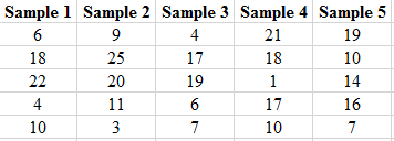
The number of females in each sample is shown below.
| Samples | Number of females | Samples | Number of females |
| Sample 1 | 2 | Sample 11 | 1 |
| Sample 2 | 1 | Sample 12 | 2 |
| Sample 3 | 2 | Sample 13 | 4 |
| Sample 4 | 3 | Sample 14 | 2 |
| Sample 5 | 1 | Sample 15 | 3 |
| Sample 6 | 2 | Sample 16 | 2 |
| Sample 7 | 3 | Sample 17 | 0 |
| Sample 8 | 1 | Sample 18 | 2 |
| Sample 9 | 1 | Sample 19 | 1 |
| Sample 10 | 2 | Sample 20 | 2 |
Explanation of Solution
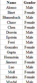
Step 1: Write the name and the gender of the club members in the Excel spreadsheet. The snapshot is shown below:
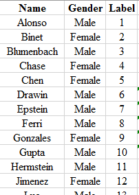
Step 2: Label each of the members using the numbers
Step 3: Use the formula

To find the number of female in each sample, the label of each female member is matched with the obtained random number of each set of sample and then the number of female is counted. The number of females obtained in each set of samples are shown in the below table.
| Samples | Number of females | Samples | Number of females |
| Sample 1 | 2 | Sample 11 | 1 |
| Sample 2 | 1 | Sample 12 | 2 |
| Sample 3 | 2 | Sample 13 | 4 |
| Sample 4 | 3 | Sample 14 | 2 |
| Sample 5 | 1 | Sample 15 | 3 |
| Sample 6 | 2 | Sample 16 | 2 |
| Sample 7 | 3 | Sample 17 | 0 |
| Sample 8 | 1 | Sample 18 | 2 |
| Sample 9 | 1 | Sample 19 | 1 |
| Sample 10 | 2 | Sample 20 | 2 |
To graph: The histogram for the number of females in each set of sample.
Explanation of Solution
Graph: To obtain the histogram for the obtained result in previous part, Excel is used. The below steps are followed to obtain the required histogram.
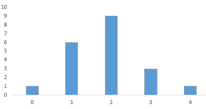
Step 1: The number of females varies from 0 to 4. The number of samples are calculated corresponding to each number of females. The number of samples with the same number of female members is clustered. The snapshot of the obtained table is shown below:
| Number of female members | Number of samples |
| 0 | 1 |
| 1 | 6 |
| 2 | 9 |
| 3 | 3 |
| 4 | 1 |
Step 2: Select the data set and go to insert and select the option of cluster column under the Recommended Charts. The screenshot is shown below:

Step 3: Click on OK. The diagram is obtained as:
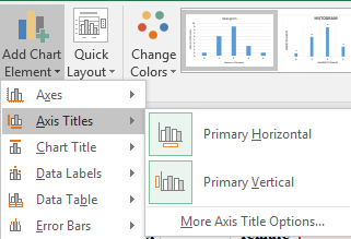
Step 4: Click on the chart area and select the option of “Primary Horizontal” and “Primary Vertical” axis under the “Add Chart Element” to add the axis title. The screenshot is shown below:
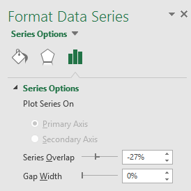
Step 5: Click on the bars of the diagrams and reduce the gap width to zero under the “Format Data Series” tab. The screenshot is shown below:
The obtained histogram is:
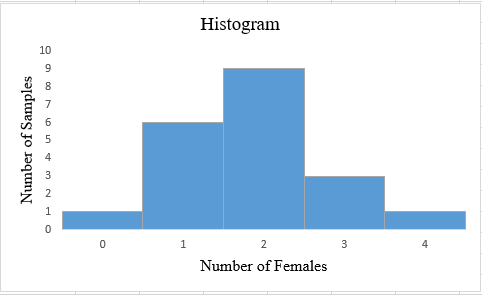
Interpretation: The obtained histogram for the number of females in each set of sample follows
To find: The average number of females in 20 samples.
Answer to Problem 13E
Solution: The average number of female is 1.85.
Explanation of Solution
Calculation:
The average number of females can be obtained by using the formula:
Hence, the average number of females is calculated as:
Therefore, the average number of females in 20 samples is 1.85.
(b)
To explain: Whether the club members should be doubtful about the discrimination if any of the five tickets does not received by women.
(b)
Answer to Problem 13E
Solution: The club member should suspect the discrimination if any of the five tickets does not received by women.
Explanation of Solution
Want to see more full solutions like this?
Chapter 3 Solutions
Statistics: Concepts and Controv. (Instructor's)


- BUSINESS DISCUSSarrow_forwardA researcher wishes to estimate, with 90% confidence, the population proportion of adults who support labeling legislation for genetically modified organisms (GMOs). Her estimate must be accurate within 4% of the true proportion. (a) No preliminary estimate is available. Find the minimum sample size needed. (b) Find the minimum sample size needed, using a prior study that found that 65% of the respondents said they support labeling legislation for GMOs. (c) Compare the results from parts (a) and (b). ... (a) What is the minimum sample size needed assuming that no prior information is available? n = (Round up to the nearest whole number as needed.)arrow_forwardThe table available below shows the costs per mile (in cents) for a sample of automobiles. At a = 0.05, can you conclude that at least one mean cost per mile is different from the others? Click on the icon to view the data table. Let Hss, HMS, HLS, Hsuv and Hмy represent the mean costs per mile for small sedans, medium sedans, large sedans, SUV 4WDs, and minivans respectively. What are the hypotheses for this test? OA. Ho: Not all the means are equal. Ha Hss HMS HLS HSUV HMV B. Ho Hss HMS HLS HSUV = μMV Ha: Hss *HMS *HLS*HSUV * HMV C. Ho Hss HMS HLS HSUV =μMV = = H: Not all the means are equal. D. Ho Hss HMS HLS HSUV HMV Ha Hss HMS HLS =HSUV = HMVarrow_forward
- Question: A company launches two different marketing campaigns to promote the same product in two different regions. After one month, the company collects the sales data (in units sold) from both regions to compare the effectiveness of the campaigns. The company wants to determine whether there is a significant difference in the mean sales between the two regions. Perform a two sample T-test You can provide your answer by inserting a text box and the answer must include: Null hypothesis, Alternative hypothesis, Show answer (output table/summary table), and Conclusion based on the P value. (2 points = 0.5 x 4 Answers) Each of these is worth 0.5 points. However, showing the calculation is must. If calculation is missing, the whole answer won't get any credit.arrow_forwardBinomial Prob. Question: A new teaching method claims to improve student engagement. A survey reveals that 60% of students find this method engaging. If 15 students are randomly selected, what is the probability that: a) Exactly 9 students find the method engaging?b) At least 7 students find the method engaging? (2 points = 1 x 2 answers) Provide answers in the yellow cellsarrow_forwardIn a survey of 2273 adults, 739 say they believe in UFOS. Construct a 95% confidence interval for the population proportion of adults who believe in UFOs. A 95% confidence interval for the population proportion is ( ☐, ☐ ). (Round to three decimal places as needed.)arrow_forward
- Find the minimum sample size n needed to estimate μ for the given values of c, σ, and E. C=0.98, σ 6.7, and E = 2 Assume that a preliminary sample has at least 30 members. n = (Round up to the nearest whole number.)arrow_forwardIn a survey of 2193 adults in a recent year, 1233 say they have made a New Year's resolution. Construct 90% and 95% confidence intervals for the population proportion. Interpret the results and compare the widths of the confidence intervals. The 90% confidence interval for the population proportion p is (Round to three decimal places as needed.) J.D) .arrow_forwardLet p be the population proportion for the following condition. Find the point estimates for p and q. In a survey of 1143 adults from country A, 317 said that they were not confident that the food they eat in country A is safe. The point estimate for p, p, is (Round to three decimal places as needed.) ...arrow_forward
- (c) Because logistic regression predicts probabilities of outcomes, observations used to build a logistic regression model need not be independent. A. false: all observations must be independent B. true C. false: only observations with the same outcome need to be independent I ANSWERED: A. false: all observations must be independent. (This was marked wrong but I have no idea why. Isn't this a basic assumption of logistic regression)arrow_forwardBusiness discussarrow_forwardSpam filters are built on principles similar to those used in logistic regression. We fit a probability that each message is spam or not spam. We have several variables for each email. Here are a few: to_multiple=1 if there are multiple recipients, winner=1 if the word 'winner' appears in the subject line, format=1 if the email is poorly formatted, re_subj=1 if "re" appears in the subject line. A logistic model was fit to a dataset with the following output: Estimate SE Z Pr(>|Z|) (Intercept) -0.8161 0.086 -9.4895 0 to_multiple -2.5651 0.3052 -8.4047 0 winner 1.5801 0.3156 5.0067 0 format -0.1528 0.1136 -1.3451 0.1786 re_subj -2.8401 0.363 -7.824 0 (a) Write down the model using the coefficients from the model fit.log_odds(spam) = -0.8161 + -2.5651 + to_multiple + 1.5801 winner + -0.1528 format + -2.8401 re_subj(b) Suppose we have an observation where to_multiple=0, winner=1, format=0, and re_subj=0. What is the predicted probability that this message is spam?…arrow_forward
 MATLAB: An Introduction with ApplicationsStatisticsISBN:9781119256830Author:Amos GilatPublisher:John Wiley & Sons Inc
 Probability and Statistics for Engineering and th...StatisticsISBN:9781305251809Author:Jay L. DevorePublisher:Cengage Learning
 Statistics for The Behavioral Sciences (MindTap C...StatisticsISBN:9781305504912Author:Frederick J Gravetter, Larry B. WallnauPublisher:Cengage Learning
 Elementary Statistics: Picturing the World (7th E...StatisticsISBN:9780134683416Author:Ron Larson, Betsy FarberPublisher:PEARSON
 The Basic Practice of StatisticsStatisticsISBN:9781319042578Author:David S. Moore, William I. Notz, Michael A. FlignerPublisher:W. H. Freeman
 Introduction to the Practice of StatisticsStatisticsISBN:9781319013387Author:David S. Moore, George P. McCabe, Bruce A. CraigPublisher:W. H. Freeman