
(a)
To make a
(a)
Answer to Problem 28.37E
Yes, the graph suggest that a multiple regression might be appropriate.
Explanation of Solution
In the question, it is given that an experiment compared the effects of adding various amounts of nitrogen fertilizers to two genotypes of tomato plants, a mild-type and a mutant variety. The percent of phosphorus in the plant, nitrogen and genotype is given in a table. Thus, the scatterplot of the amount of phosphorus in the plant against nitrogen, using different symbols for the two plant genotype is as follows:
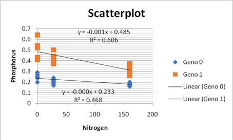
In the scatterplot, we can see that the genotype zero is in red color and genotype one is in blue color. And the lines in the scatterplot are almost parallel so it is linear in nature and in both the lines the points are moving downwards so they are negative in relationship. Thus, as they are parallel so the graph suggest that a multiple regression might be appropriate for these data.
(b)
To use a software to obtain the estimated multiple linear regression equation when the two explanatory variables nitrogen and genotype are included and create a residual plot and explain are the conditions for multiple linear regression satisfied.
(b)
Answer to Problem 28.37E
The estimated multiple linear regression equation is
Explanation of Solution
In the question, it is given that an experiment compared the effects of adding various amounts of nitrogen fertilizers to two genotypes of tomato plants, a mild-type and a mutant variety. The percent of phosphorus in the plant, nitrogen and genotype is given in a table. Now, we will use the Excel to obtain the estimated multiple linear regression equation when the two explanatory variables nitrogen and genotype are included and also the residual plot is constructed. We will use the option data analysis in the data tab and run the
| ANOVA | |||||
| df | SS | MS | F | Significance F | |
| Regression | 2 | 0.46916 | 0.23458 | 76.2375 | 4.25E-13 |
| Residual | 33 | 0.10154 | 0.003077 | ||
| Total | 35 | 0.5707 |
| Coefficients | Standard Error | t Stat | P-value | |
| Intercept | 0.256853 | 0.015489 | 16.58326 | 1.43E-17 |
| Nitrogen | -0.00071 | 0.000133 | -5.37461 | 6.11E-06 |
| Genotype | 0.205556 | 0.01849 | 11.11704 | 1.07E-12 |
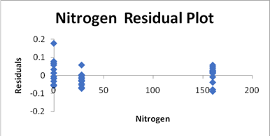
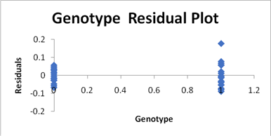
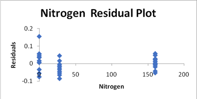
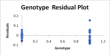
The residual plot will be constructed as:
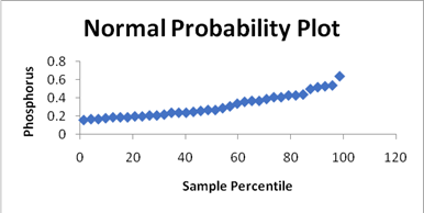
And the normal plot will be constructed as:
Now, the estimated multiple linear regression equation when the two explanatory variables nitrogen and genotype are included is as:
Where
(c)
To create a new variable called interaction by multiplying the explanatory variables nitrogen and genotype and add this new variable to your regression model and provide the estimated multiple linear regression equation and create regression plot for this and discuss whether the conditions for multiple linear regression are met.
(c)
Answer to Problem 28.37E
The conditions for multiple linear regression are met and the estimated multiple linear regression equation is
Explanation of Solution
In the question, it is given that an experiment compared the effects of adding various amounts of nitrogen fertilizers to two genotypes of tomato plants, a mild-type and a mutant variety. The percent of phosphorus in the plant, nitrogen and genotype is given in a table. And a new variable called interaction is created by multiplying the explanatory variables nitrogen and genotype. Now, we will use the Excel to obtain the estimated multiple linear regression equation when the two explanatory variables nitrogen and genotype and the interaction are included and also the residual plot is constructed. We will use the option data analysis in the data tab and run the regression analysis. The result will be as:
| ANOVA | |||||
| df | SS | MS | F | Significance F | |
| Regression | 3 | 0.49273 | 0.164243 | 67.4079 | 6.35E-14 |
| Residual | 32 | 0.07797 | 0.002437 | ||
| Total | 35 | 0.5707 |
| Coefficients | Standard Error | t Stat | P-value | |
| Intercept | 0.23387 | 0.015639 | 14.95438 | 5.42E-16 |
| Nitrogen | -0.00035 | 0.000167 | -2.0715 | 0.046455 |
| Genotype | 0.251522 | 0.022117 | 11.37245 | 8.91E-13 |
| Interaction | -0.00073 | 0.000236 | -3.11022 | 0.003912 |
The residual plot is as follows:
The normal plot is as follows:

Now, the estimated multiple linear regression equation when the two explanatory variables nitrogen and genotype and interaction are included is as:
Where
(d)
To explain does the ANOVA table for the model with the interaction term indicate that at least one of the explanatory variables is helpful in predicting the amount of phosphorus in the plant and explain do the individual t tests indicate that all coefficients are significantly different from zero.
(d)
Answer to Problem 28.37E
Yes, the ANOVA table for the model with the interaction term indicates that at least one of the explanatory variables is helpful in predicting the amount of phosphorus in the plant and the individual t tests indicate that all coefficients are significantly different from zero.
Explanation of Solution
In the question, it is given that an experiment compared the effects of adding various amounts of nitrogen fertilizers to two genotypes of tomato plants, a mild-type and a mutant variety. The percent of phosphorus in the plant, nitrogen and genotype is given in a table. Since in the ANOVA table in part (c) we can see that the P-value is less than the level of significance,
Thus, we can say that the ANOVA table for the model with the interaction term indicates that at least one of the explanatory variables is helpful in predicting the amount of phosphorus in the plant. And as we can see in the result of the regression analysis in part (c), we can see that all the P-values are less than the level of significance i.e.
Thus, we have sufficient evidence to conclude that the individual t tests indicate that all coefficients are significantly different from zero.
Want to see more full solutions like this?
Chapter 28 Solutions
EBK PRACTICE OF STATISTICS IN THE LIFE

- ian income of $50,000. erty rate of 13. Using data from 50 workers, a researcher estimates Wage = Bo+B,Education + B₂Experience + B3Age+e, where Wage is the hourly wage rate and Education, Experience, and Age are the years of higher education, the years of experience, and the age of the worker, respectively. A portion of the regression results is shown in the following table. ni ogolloo bash 1 Standard Coefficients error t stat p-value Intercept 7.87 4.09 1.93 0.0603 Education 1.44 0.34 4.24 0.0001 Experience 0.45 0.14 3.16 0.0028 Age -0.01 0.08 -0.14 0.8920 a. Interpret the estimated coefficients for Education and Experience. b. Predict the hourly wage rate for a 30-year-old worker with four years of higher education and three years of experience.arrow_forward1. If a firm spends more on advertising, is it likely to increase sales? Data on annual sales (in $100,000s) and advertising expenditures (in $10,000s) were collected for 20 firms in order to estimate the model Sales = Po + B₁Advertising + ε. A portion of the regression results is shown in the accompanying table. Intercept Advertising Standard Coefficients Error t Stat p-value -7.42 1.46 -5.09 7.66E-05 0.42 0.05 8.70 7.26E-08 a. Interpret the estimated slope coefficient. b. What is the sample regression equation? C. Predict the sales for a firm that spends $500,000 annually on advertising.arrow_forwardCan you help me solve problem 38 with steps im stuck.arrow_forward
- How do the samples hold up to the efficiency test? What percentages of the samples pass or fail the test? What would be the likelihood of having the following specific number of efficiency test failures in the next 300 processors tested? 1 failures, 5 failures, 10 failures and 20 failures.arrow_forwardThe battery temperatures are a major concern for us. Can you analyze and describe the sample data? What are the average and median temperatures? How much variability is there in the temperatures? Is there anything that stands out? Our engineers’ assumption is that the temperature data is normally distributed. If that is the case, what would be the likelihood that the Safety Zone temperature will exceed 5.15 degrees? What is the probability that the Safety Zone temperature will be less than 4.65 degrees? What is the actual percentage of samples that exceed 5.25 degrees or are less than 4.75 degrees? Is the manufacturing process producing units with stable Safety Zone temperatures? Can you check if there are any apparent changes in the temperature pattern? Are there any outliers? A closer look at the Z-scores should help you in this regard.arrow_forwardNeed help pleasearrow_forward
- Please conduct a step by step of these statistical tests on separate sheets of Microsoft Excel. If the calculations in Microsoft Excel are incorrect, the null and alternative hypotheses, as well as the conclusions drawn from them, will be meaningless and will not receive any points. 4. One-Way ANOVA: Analyze the customer satisfaction scores across four different product categories to determine if there is a significant difference in means. (Hints: The null can be about maintaining status-quo or no difference among groups) H0 = H1=arrow_forwardPlease conduct a step by step of these statistical tests on separate sheets of Microsoft Excel. If the calculations in Microsoft Excel are incorrect, the null and alternative hypotheses, as well as the conclusions drawn from them, will be meaningless and will not receive any points 2. Two-Sample T-Test: Compare the average sales revenue of two different regions to determine if there is a significant difference. (Hints: The null can be about maintaining status-quo or no difference among groups; if alternative hypothesis is non-directional use the two-tailed p-value from excel file to make a decision about rejecting or not rejecting null) H0 = H1=arrow_forwardPlease conduct a step by step of these statistical tests on separate sheets of Microsoft Excel. If the calculations in Microsoft Excel are incorrect, the null and alternative hypotheses, as well as the conclusions drawn from them, will be meaningless and will not receive any points 3. Paired T-Test: A company implemented a training program to improve employee performance. To evaluate the effectiveness of the program, the company recorded the test scores of 25 employees before and after the training. Determine if the training program is effective in terms of scores of participants before and after the training. (Hints: The null can be about maintaining status-quo or no difference among groups; if alternative hypothesis is non-directional, use the two-tailed p-value from excel file to make a decision about rejecting or not rejecting the null) H0 = H1= Conclusion:arrow_forward
- Please conduct a step by step of these statistical tests on separate sheets of Microsoft Excel. If the calculations in Microsoft Excel are incorrect, the null and alternative hypotheses, as well as the conclusions drawn from them, will be meaningless and will not receive any points. The data for the following questions is provided in Microsoft Excel file on 4 separate sheets. Please conduct these statistical tests on separate sheets of Microsoft Excel. If the calculations in Microsoft Excel are incorrect, the null and alternative hypotheses, as well as the conclusions drawn from them, will be meaningless and will not receive any points. 1. One Sample T-Test: Determine whether the average satisfaction rating of customers for a product is significantly different from a hypothetical mean of 75. (Hints: The null can be about maintaining status-quo or no difference; If your alternative hypothesis is non-directional (e.g., μ≠75), you should use the two-tailed p-value from excel file to…arrow_forwardPlease conduct a step by step of these statistical tests on separate sheets of Microsoft Excel. If the calculations in Microsoft Excel are incorrect, the null and alternative hypotheses, as well as the conclusions drawn from them, will be meaningless and will not receive any points. 1. One Sample T-Test: Determine whether the average satisfaction rating of customers for a product is significantly different from a hypothetical mean of 75. (Hints: The null can be about maintaining status-quo or no difference; If your alternative hypothesis is non-directional (e.g., μ≠75), you should use the two-tailed p-value from excel file to make a decision about rejecting or not rejecting null. If alternative is directional (e.g., μ < 75), you should use the lower-tailed p-value. For alternative hypothesis μ > 75, you should use the upper-tailed p-value.) H0 = H1= Conclusion: The p value from one sample t-test is _______. Since the two-tailed p-value is _______ 2. Two-Sample T-Test:…arrow_forwardPlease conduct a step by step of these statistical tests on separate sheets of Microsoft Excel. If the calculations in Microsoft Excel are incorrect, the null and alternative hypotheses, as well as the conclusions drawn from them, will be meaningless and will not receive any points. What is one sample T-test? Give an example of business application of this test? What is Two-Sample T-Test. Give an example of business application of this test? .What is paired T-test. Give an example of business application of this test? What is one way ANOVA test. Give an example of business application of this test? 1. One Sample T-Test: Determine whether the average satisfaction rating of customers for a product is significantly different from a hypothetical mean of 75. (Hints: The null can be about maintaining status-quo or no difference; If your alternative hypothesis is non-directional (e.g., μ≠75), you should use the two-tailed p-value from excel file to make a decision about rejecting or not…arrow_forward
 MATLAB: An Introduction with ApplicationsStatisticsISBN:9781119256830Author:Amos GilatPublisher:John Wiley & Sons Inc
 Probability and Statistics for Engineering and th...StatisticsISBN:9781305251809Author:Jay L. DevorePublisher:Cengage Learning
 Statistics for The Behavioral Sciences (MindTap C...StatisticsISBN:9781305504912Author:Frederick J Gravetter, Larry B. WallnauPublisher:Cengage Learning
 Elementary Statistics: Picturing the World (7th E...StatisticsISBN:9780134683416Author:Ron Larson, Betsy FarberPublisher:PEARSON
 The Basic Practice of StatisticsStatisticsISBN:9781319042578Author:David S. Moore, William I. Notz, Michael A. FlignerPublisher:W. H. Freeman
 Introduction to the Practice of StatisticsStatisticsISBN:9781319013387Author:David S. Moore, George P. McCabe, Bruce A. CraigPublisher:W. H. Freeman