
To determine: The aggregate consumer function, income-expenditure equilibrium and the value of the multiplier.
Concept Introduction:
The formula to calculate change in GDP is:
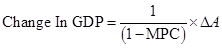
Here,
 is autonomous spending.
 - MPC is marginal propensity to consume.
Marginal Propensity to Consume (MPC): It is defined as the change which occurs in total consumption level due to a change in disposable income.
The formula to calculate MPC is:

Here,
 is change in disposable income.
  is change in consumption level.
 - MPC is marginal propensity to consume.
Multiplier: It is defined as the ratio of total change in the gross domestic product due to a change in the autonomous spending.
The formula to calculate multiplier is:
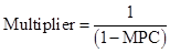
Here,
- MPC is marginal propensity to consume.
Consumption Level (C): It is one of the largest components of GD .The individual consumption depends on the disposable income.
Consumption Function: It shows how the change in disposable income of an individual changes the consumption level.
The formula to calculate consumption function is:
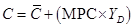
Here,
- C is consumption level.
 is autonomous consumption.
  is disposable income.
 - MPC is marginal propensity to consume.
Autonomous Consumption: This is defined as the consumption level when the income of an individual is zero.
Planned Aggregate Spending: It is the summation of consumption level in an economy and the planned investment.
The formula to calculate planned aggregate spending is:
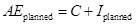
Here,
- C is consumption level.
 is the planned investment spending.
  is the planned aggregate spending.
Unplanned Investment: All those investments that businesses do not intend to take in a given time. It is certain due to some external factors like fall in interest rate and increase in future profitability.
The formula to calculate unplanned investment is:
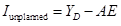
Here,
- YDis disposable income.
 is unplanned investment spending.
 - AE is the planned aggregate spending.
Explanation of Solution
a. Planned aggregate expenditure and unplanned investment.
| GDP | YD(A) | C(B) | Iplanned(C) | AEplanned(D) | Iunplanned |
| (billions of dollars) | |||||
| 0 | 0 | 100 | 300 | 400 |  |
| 400 | 400 | 400 | 300 | 700 |  |
| 800 | 800 | 700 | 300 | 1,000 |  |
| 1,200 | 1,200 | 1,000 | 300 | 1,300 |  |
| 1,600 | 1,600 | 1,300 | 300 | 1,600 | 0 |
| 2,000 | 2,000 | 1,600 | 300 | 1,900 | 100 |
| 2,400 | 2,400 | 1,900 | 300 | 2,200 | 200 |
| 2,800 | 2,800 | 2,200 | 300 | 2,500 | 300 |
| 3,200 | 3,200 | 2,500 | 300 | 2,800 | 400 |
Conclusion:
Hence, the unplanned investment and the planned aggregate expenditure at specific income level have been stated in the table.
b. Aggregate consumption function.
Given,
Autonomous consumption is $100 billion.
Change in disposable income is $400 billion.
Change in aggregate consumer spending is $300 billion.
The formula to calculate MPC is:

Substitute $300 billion for  and $400 billion for
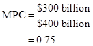
Hence MPC is 0.75.
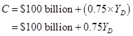
The formula to calculate consumption function is:
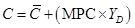
Substitute $100 billion for  and 0.75 for MPC:
Conclusion:
Thus, the Consumption function is 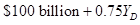
c. Income-expenditure equilibrium GDP.
- Income expenditure equilibrium GDP is the point where planned aggregate spending is equal to the GDP.
- The table in part a highlights that the condition is satisfied at the level where GDP is equal to $1,600 billion.
Conclusion:
Hence, the equilibrium GDP (Y*) is $1,600 billion.
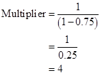
d. Value of the multiplier:
Given,
MPC is 0.75
The formula to calculate multiplier is:
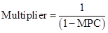
Substitute 0.75 for MPC:
Conclusion;
Thus, multiplier is 4.
e. The new Y* when planned investment changes.
Given,
New investment is $200 billion
Initial investment is $300 billion
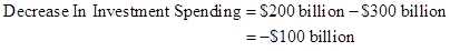
The formula to calculate change in planned investment is:

Substitute $200 billion for new investment and $200 billion for initial investment:
Given,
Change in investment is  billion.
Real GDP is $1,600 billion.
Multiplier is 4.
The formula to calculate new Y* is:

Substitute $1,600 billion for real GDP, 4 for multiplier and  billion for change in investment:
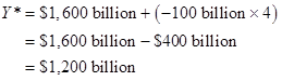
Conclusion:
Thus, new Y* is $1,200 billion.
f. The new Y* when autonomous consumption changes.
Given,
New autonomous consumption is $200 billion.
Initial autonomous consumption is $100 billion.
The formula to calculate change in autonomous consumption is:
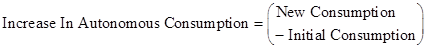
Substitute $200 billion for new consumption and $100 billion for initial consumption:
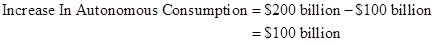
Given,
Change in consumption is $100 billion.
Real GDP is $1,600 billion.
Multiplier is 4.
The formula to calculate new Y* is:

Substitute $1,600 billion for real GDP, 4 for multiplier and $100 billion for change in consumption:
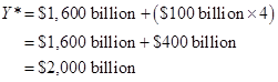
Conclusion:
Thus, new Y* is $2,000 billion.
Want to see more full solutions like this?

- Do they have any specified areas of interest( examples: oil/gas, education, subsistence). Please provide the answer to the question using www.akleg.gov for Senate Bill 30?arrow_forwardA brief synopsis of whether you believe they represent your interest, why or why not? Please provide the answer to this question by using www.akleg for senate bill 30 ?arrow_forwardWhat is their background (degree, career/job, community of origin, anything else you choose to include) Please provide the answers using www.akleg.gov for Senate Bill 30?arrow_forward
- Please provide the answer to these questions using informatioin from www.akleg.gov for Senate bill 30. What is their party affiliation?arrow_forwardPlease provide the answer to the question using information from www.akleg.gov for Senate Bill 30. How lonng have they been in public office?arrow_forwardPlease provide the answer to the following questions using www.akleg.gov website for Senate Bill 30. What District do they represent?arrow_forward
- Please provide the answer to this question using www.akleg.gov for Senate Bill 30? Do they hold any committe seats?arrow_forwardWhat impact does the North American Free Trade Agreement have on relations between countries in North America? NAFTA regulates and enforces protections for workers to ensure that they have safe working environments and fair wages. NAFTA eliminates tariffs and trade restrictions, facilitating export and import between countries in North America. NAFTA sets up regulations limiting industrial pollution in all three countries, ensuring the costs of manufacturing are similar in each country. NAFTA eliminates trade restrictions on products from embargoed countries.arrow_forwardWhich of the following is included in the GDP_________? Group of answer choices The two answers describe components of the GDP. The federal government expenditure on welfare payments. Households goods and services produced at home. Neither of the two answers describe components of the GDP.arrow_forward
- What are two examples of where historical cost is used within the financial statements. State both the account name and the amount for each account selected. What was the amount of revenue that Airbnb reported for 2024? Did the revenue grow over the prior year of 2023? What was the dollar and the percentage increase or decrease?arrow_forwardWhat was the amount of revenue that Airbnb reported for 2024? Did the revenue grow over the prior year of 2023? What was the dollar and the percentage increase or decrease? What was the amount of net income or net loss that Airbnb reported for the year of 2024? Did the net income increase or decrease versus the prior year of 2023? What was the dollar and the percentage increase or decrease?arrow_forwardWho are the Airbnb's independent auditors and what is the role of these auditors? What opinion do the Airbnb independent auditors express regarding the financial statements and what does this opinion mean to an investor?arrow_forward

 Principles of Economics (12th Edition)EconomicsISBN:9780134078779Author:Karl E. Case, Ray C. Fair, Sharon E. OsterPublisher:PEARSON
 Engineering Economy (17th Edition)EconomicsISBN:9780134870069Author:William G. Sullivan, Elin M. Wicks, C. Patrick KoellingPublisher:PEARSON
 Principles of Economics (MindTap Course List)EconomicsISBN:9781305585126Author:N. Gregory MankiwPublisher:Cengage Learning
 Managerial Economics: A Problem Solving ApproachEconomicsISBN:9781337106665Author:Luke M. Froeb, Brian T. McCann, Michael R. Ward, Mike ShorPublisher:Cengage Learning
 Managerial Economics & Business Strategy (Mcgraw-...EconomicsISBN:9781259290619Author:Michael Baye, Jeff PrincePublisher:McGraw-Hill Education