
To determine: The aggregate consumer function, income-expenditure equilibrium and the value of the multiplier.
Concept Introduction:
The formula to calculate change in GDP is:
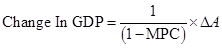
Here,
 is autonomous spending.
 - MPC is marginal propensity to consume.
Marginal Propensity to Consume (MPC): It is defined as the change which occurs in total consumption level due to a change in disposable income.
The formula to calculate MPC is:

Here,
 is change in disposable income.
  is change in consumption level.
 - MPC is marginal propensity to consume.
Multiplier: It is defined as the ratio of total change in the gross domestic product due to a change in the autonomous spending.
The formula to calculate multiplier is:
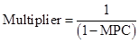
Here,
- MPC is marginal propensity to consume.
Consumption Level (C): It is one of the largest components of GD .The individual consumption depends on the disposable income.
Consumption Function: It shows how the change in disposable income of an individual changes the consumption level.
The formula to calculate consumption function is:
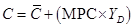
Here,
- C is consumption level.
 is autonomous consumption.
  is disposable income.
 - MPC is marginal propensity to consume.
Autonomous Consumption: This is defined as the consumption level when the income of an individual is zero.
Planned Aggregate Spending: It is the summation of consumption level in an economy and the planned investment.
The formula to calculate planned aggregate spending is:
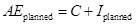
Here,
- C is consumption level.
 is the planned investment spending.
  is the planned aggregate spending.
Unplanned Investment: All those investments that businesses do not intend to take in a given time. It is certain due to some external factors like fall in interest rate and increase in future profitability.
The formula to calculate unplanned investment is:
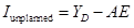
Here,
- YDis disposable income.
 is unplanned investment spending.
 - AE is the planned aggregate spending.
Explanation of Solution
a. Planned aggregate expenditure and unplanned investment.
| GDP | YD(A) | C(B) | Iplanned(C) | AEplanned(D) | Iunplanned |
| (billions of dollars) | |||||
| 0 | 0 | 100 | 300 | 400 |  |
| 400 | 400 | 400 | 300 | 700 |  |
| 800 | 800 | 700 | 300 | 1,000 |  |
| 1,200 | 1,200 | 1,000 | 300 | 1,300 |  |
| 1,600 | 1,600 | 1,300 | 300 | 1,600 | 0 |
| 2,000 | 2,000 | 1,600 | 300 | 1,900 | 100 |
| 2,400 | 2,400 | 1,900 | 300 | 2,200 | 200 |
| 2,800 | 2,800 | 2,200 | 300 | 2,500 | 300 |
| 3,200 | 3,200 | 2,500 | 300 | 2,800 | 400 |
Conclusion:
Hence, the unplanned investment and the planned aggregate expenditure at specific income level have been stated in the table.
b. Aggregate consumption function.
Given,
Autonomous consumption is $100 billion.
Change in disposable income is $400 billion.
Change in aggregate consumer spending is $300 billion.
The formula to calculate MPC is:

Substitute $300 billion for  and $400 billion for
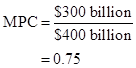
Hence MPC is 0.75.
The formula to calculate consumption function is:
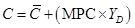
Substitute $100 billion for  and 0.75 for MPC:
Conclusion:
Thus, the Consumption function is 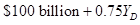
c. Income-expenditure equilibrium GDP.
- Income expenditure equilibrium GDP is the point where planned aggregate spending is equal to the GDP.
- The table in part a highlights that the condition is satisfied at the level where GDP is equal to $1,600 billion.
Conclusion:
Hence, the equilibrium GDP (Y*) is $1,600 billion.
d. Value of the multiplier:
Given,
MPC is 0.75
The formula to calculate multiplier is:
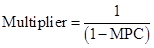
Substitute 0.75 for MPC:
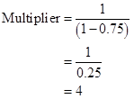
Conclusion;
Thus, multiplier is 4.
e. The new Y* when planned investment changes.
Given,
New investment is $200 billion
Initial investment is $300 billion
The formula to calculate change in planned investment is:

Substitute $200 billion for new investment and $200 billion for initial investment:
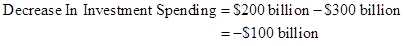
Given,
Change in investment is  billion.
Real GDP is $1,600 billion.
Multiplier is 4.
The formula to calculate new Y* is:

Substitute $1,600 billion for real GDP, 4 for multiplier and  billion for change in investment:
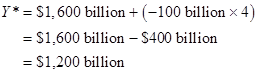
Conclusion:
Thus, new Y* is $1,200 billion.
f. The new Y* when autonomous consumption changes.
Given,
New autonomous consumption is $200 billion.
Initial autonomous consumption is $100 billion.
The formula to calculate change in autonomous consumption is:
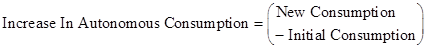
Substitute $200 billion for new consumption and $100 billion for initial consumption:
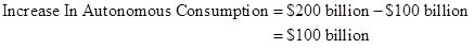
Given,
Change in consumption is $100 billion.
Real GDP is $1,600 billion.
Multiplier is 4.
The formula to calculate new Y* is:

Substitute $1,600 billion for real GDP, 4 for multiplier and $100 billion for change in consumption:
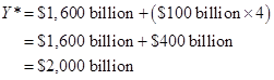
Conclusion:
Thus, new Y* is $2,000 billion.
Want to see more full solutions like this?

- After the ban is imposed, Joe’s firm switches to the more expensive biodegradable disposable cups. This increases the cost associated with each cup of coffee it produces. Which cost curve(s) will be impacted by the use of the more expensive biodegradable disposable cups? Why? Which cost curve(s) will not shift, and why not? Please use the table below to answer this question. For the second column (“Impacted? If so, how?”), please use one of the following three choices: No shift; Shifts up (i.e., increases: at nearly any given quantity, the cost goes up); or Shifts down (i.e., decreases: at nearly any given quantity, the cost goes down). $ Cost Curve Impacted? If so, how? Explanation of the Shift: Why or Why Not AFC No shift. Fix costs stay the same, regardless of quantity. Fixed cost is calculated as Fixed Cost/Quantity. Since fixed costs remain unchanged, AFC stays the same for each quantity. MC Shifts up. Since the biodegradable cups are more expensive, the…arrow_forwardStyrofoam is non-biodegradable and is not easily recyclable. Many cities and at least one state have enacted laws that ban the use of polystyrene containers. These locales understand that banning these containers will force many businesses to turn to other more expensive forms of packaging and cups, but argue the ban is environmentally important. Shane owns a firm with a conventional production function resulting in U-shaped ATC, AVC, and MC curves. Shane's business sells takeout food and drinks that are currently packaged in styrofoam containers and cups. Graph the short-run AFC0, AVC0, ATC0, and MC0 curves for Shane's firm before the ban on using styrofoam containers.arrow_forwardd-farrow_forward
- a-c pleasearrow_forwardd-farrow_forwardPART II: Multipart Problems wood or solem of triflussd aidi 1. Assume that a society has a polluting industry comprising two firms, where the industry-level marginal abatement cost curve is given by: MAC = 24 - ()E and the marginal damage function is given by: MDF = 2E. What is the efficient level of emissions? b. What constant per-unit emissions tax could achieve the efficient emissions level? points) c. What is the net benefit to society of moving from the unregulated emissions level to the efficient level? In response to industry complaints about the costs of the tax, a cap-and-trade program is proposed. The marginal abatement cost curves for the two firms are given by: MAC=24-E and MAC2 = 24-2E2. d. How could a cap-and-trade program that achieves the same level of emissions as the tax be designed to reduce the costs of regulation to the two firms?arrow_forward
- Only #4 please, Use a graph please if needed to help provearrow_forwarda-carrow_forwardFor these questions, you must state "true," "false," or "uncertain" and argue your case (roughly 3 to 5 sentences). When appropriate, the use of graphs will make for stronger answers. Credit will depend entirely on the quality of your explanation. 1. If the industry facing regulation for its pollutant emissions has a lot of political capital, direct regulatory intervention will be more viable than an emissions tax to address this market failure. 2. A stated-preference method will provide a measure of the value of Komodo dragons that is more accurate than the value estimated through application of the travel cost model to visitation data for Komodo National Park in Indonesia. 3. A correlation between community demographics and the present location of polluting facilities is sufficient to claim a violation of distributive justice. olsvrc Q 4. When the damages from pollution are uncertain, a price-based mechanism is best equipped to manage the costs of the regulator's imperfect…arrow_forward
- For environmental economics, question number 2 only please-- thank you!arrow_forwardFor these questions, you must state "true," "false," or "uncertain" and argue your case (roughly 3 to 5 sentences). When appropriate, the use of graphs will make for stronger answers. Credit will depend entirely on the quality of your explanation. 1. If the industry facing regulation for its pollutant emissions has a lot of political capital, direct regulatory intervention will be more viable than an emissions tax to address this market failure. cullog iba linevoz ve bubivorearrow_forwardExercise 3 The production function of a firm is described by the following equation Q=10,000-3L2 where L stands for the units of labour. a) Draw a graph for this equation. Use the quantity produced in the y-axis, and the units of labour in the x-axis. b) What is the maximum production level? c) How many units of labour are needed at that point? d) Provide one reference with you answer.arrow_forward

 Principles of Economics (12th Edition)EconomicsISBN:9780134078779Author:Karl E. Case, Ray C. Fair, Sharon E. OsterPublisher:PEARSON
 Engineering Economy (17th Edition)EconomicsISBN:9780134870069Author:William G. Sullivan, Elin M. Wicks, C. Patrick KoellingPublisher:PEARSON
 Principles of Economics (MindTap Course List)EconomicsISBN:9781305585126Author:N. Gregory MankiwPublisher:Cengage Learning
 Managerial Economics: A Problem Solving ApproachEconomicsISBN:9781337106665Author:Luke M. Froeb, Brian T. McCann, Michael R. Ward, Mike ShorPublisher:Cengage Learning
 Managerial Economics & Business Strategy (Mcgraw-...EconomicsISBN:9781259290619Author:Michael Baye, Jeff PrincePublisher:McGraw-Hill Education