
Concept explainers
Videos
Solve the following initial value problem over the interval from
(a) Analytically.
(b) Euler's method with
(c) Midpoint method with
(d) Fourth-order RK method with
(a)
To calculate: The solution of the initial value problem
Answer to Problem 1P
Solution:
The solution to the initial value problem is
Explanation of Solution
Given Information:
The initial value problem
Formula used:
Tosolve an initial value problem of the form
Calculation:
Rewrite the provided differential equation as,
Integrate both sides to get,
Now use the initial condition
Hence, the analytical solution of the initial value problem is
(b)
To calculate: The solution of the initial value problem
Answer to Problem 1P
Solution:
For
| t | y | |
| 0 | 1 | |
| 0.5 | 0.45 | |
| 1 | 0.25875 | |
| 1.5 | 0.245813 | 0.282684 |
| 2 | 0.387155 | 1.122749 |
And, for
| t | y | |
| 0 | 1 | |
| 0.25 | 0.725 | |
| 0.5 | 0.536593 | |
| 0.75 | 0.422861 | |
| 1 | 0.36603 | |
| 1.25 | 0.356879 | 0.165057 |
| 1.5 | 0.398143 | 0.457865 |
| 1.75 | 0.51261 | 1.005997 |
| 2 | 0.764109 | 2.215916 |
Explanation of Solution
Given Information:
The initial value problem
Formula used:
Solve an initial value problem of the form
Calculation:
From the initial condition
Let
Proceed further and use the following MATLAB code to implement Euler’s method and solve the differential equation.
Execute the above code to obtain the solutions for
| t | y | |
| 0 | 1 | |
| 0.5 | 0.45 | |
| 1 | 0.25875 | |
| 1.5 | 0.245813 | 0.282684 |
| 2 | 0.387155 | 1.122749 |
Now, the similar procedure can be followedfor the step size
The results thus obtained are tabulated as,
| t | y | |
| 0 | 1 | |
| 0.25 | 0.725 | |
| 0.5 | 0.536593 | |
| 0.75 | 0.422861 | |
| 1 | 0.36603 | |
| 1.25 | 0.356879 | 0.165057 |
| 1.5 | 0.398143 | 0.457865 |
| 1.75 | 0.51261 | 1.005997 |
| 2 | 0.764109 | 2.215916 |
The results for the two-step-sizes are plotted along with the analytical solution
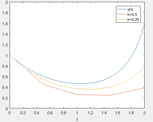
It is inferred that the smaller step-size would give a better approximation to the solution.
(c)
To calculate: The solution of the initial value problem
Answer to Problem 1P
Solution:
The solutions are tabulated as,
| t | y | |
| 0 | 1 | |
| 0.5 | 0.623906 | |
| 1 | 0.491862 | |
| 1.5 | 0.602762 | 0.693176 |
| 2 | 1.364267 | 3.956374 |
Explanation of Solution
Given Information:
The initial value problem
Formula used:
Solve an initial value problem of the form
Here,
Calculation:
From the initial condition
Let
Now,
Proceed further and use the following MATLAB code to implement mid-point iterative scheme and solve the differential equation.
Execute the above code to obtain the solutions tabulated as,
| t | Y | |
| 0 | 1 | |
| 0.5 | 0.623906 | |
| 1 | 0.491862 | |
| 1.5 | 0.602762 | 0.693176 |
| 2 | 1.364267 | 3.956374 |
The results for the are plotted along with the analytical solution
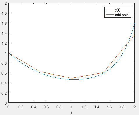
Thus, it is inferred that the mid-point method gives a good approximation to the solution.
(d)
To calculate: The solution of the initial value problem
Answer to Problem 1P
Solution:
The solutions are tabulated as,
| t | y | ||||
| 0 | 1 | ||||
| 0.5 | 0.6016 | ||||
| 1 | 0.4645 | 0.2095 | 0.2391 | 0.6717 | |
| 1.5 | 0.5914 | 0.6801 | 1.4953 | 1.8937 | 4.4609 |
| 2 | 1.5845 | 4.5949 | 10.8302 | 17.0071 | 51.9532 |
Explanation of Solution
Given Information:
The initial value problem
Formula used:
Solve an initial value problem of the form
In the above expression,
Calculation:
From the initial condition
Let
And,
And,
Therefore,
Proceed further and use the following MATLAB code to implement RK method of order four, solve the differential equation.
In an another .m file, define the equation as,
Execute the above code to obtain the solutions tabulated as,
| t | y | ||||
| 0 | 1 | ||||
| 0.5 | 0.6016 | ||||
| 1 | 0.4645 | 0.2095 | 0.2391 | 0.6717 | |
| 1.5 | 0.5914 | 0.6801 | 1.4953 | 1.8937 | 4.4609 |
| 2 | 1.5845 | 4.5949 | 10.8302 | 17.0071 | 51.9532 |
The results for the are plotted along with the analytical solution
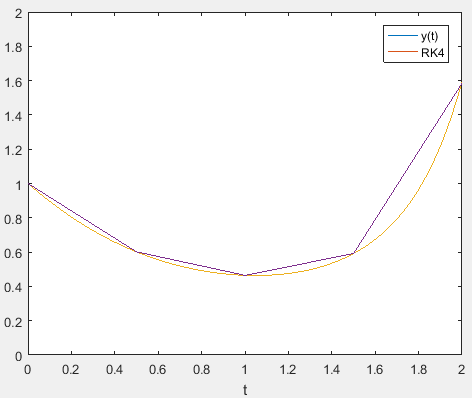
Hence, it is inferred that the RK method of order four gives the best approximation to the solution.
Want to see more full solutions like this?
Chapter 25 Solutions
Numerical Methods for Engineers


- 2. Figure below shows a U-tube manometer open at both ends and containing a column of liquid mercury of length l and specific weight y. Considering a small displacement x of the manometer meniscus from its equilibrium position (or datum), determine the equivalent spring constant associated with the restoring force. Datum Area, Aarrow_forward1. The consequences of a head-on collision of two automobiles can be studied by considering the impact of the automobile on a barrier, as shown in figure below. Construct a mathematical model (i.e., draw the diagram) by considering the masses of the automobile body, engine, transmission, and suspension and the elasticity of the bumpers, radiator, sheet metal body, driveline, and engine mounts.arrow_forward3.) 15.40 – Collar B moves up at constant velocity vB = 1.5 m/s. Rod AB has length = 1.2 m. The incline is at angle = 25°. Compute an expression for the angular velocity of rod AB, ė and the velocity of end A of the rod (✓✓) as a function of v₂,1,0,0. Then compute numerical answers for ȧ & y_ with 0 = 50°.arrow_forward
- 2.) 15.12 The assembly shown consists of the straight rod ABC which passes through and is welded to the grectangular plate DEFH. The assembly rotates about the axis AC with a constant angular velocity of 9 rad/s. Knowing that the motion when viewed from C is counterclockwise, determine the velocity and acceleration of corner F.arrow_forward500 Q3: The attachment shown in Fig.3 is made of 1040 HR. The static force is 30 kN. Specify the weldment (give the pattern, electrode number, type of weld, length of weld, and leg size). Fig. 3 All dimension in mm 30 kN 100 (10 Marks)arrow_forward(read image) (answer given)arrow_forward
- A cylinder and a disk are used as pulleys, as shown in the figure. Using the data given in the figure, if a body of mass m = 3 kg is released from rest after falling a height h 1.5 m, find: a) The velocity of the body. b) The angular velocity of the disk. c) The number of revolutions the cylinder has made. T₁ F Rd = 0.2 m md = 2 kg T T₂1 Rc = 0.4 m mc = 5 kg ☐ m = 3 kgarrow_forward(read image) (answer given)arrow_forward11-5. Compute all the dimensional changes for the steel bar when subjected to the loads shown. The proportional limit of the steel is 230 MPa. 265 kN 100 mm 600 kN 25 mm thickness X Z 600 kN 450 mm E=207×103 MPa; μ= 0.25 265 kNarrow_forward
- T₁ F Rd = 0.2 m md = 2 kg T₂ Tz1 Rc = 0.4 m mc = 5 kg m = 3 kgarrow_forward2. Find a basis of solutions by the Frobenius method. Try to identify the series as expansions of known functions. (x + 2)²y" + (x + 2)y' - y = 0 ; Hint: Let: z = x+2arrow_forward1. Find a power series solution in powers of x. y" - y' + x²y = 0arrow_forward
 Elements Of ElectromagneticsMechanical EngineeringISBN:9780190698614Author:Sadiku, Matthew N. O.Publisher:Oxford University Press
 Mechanics of Materials (10th Edition)Mechanical EngineeringISBN:9780134319650Author:Russell C. HibbelerPublisher:PEARSON
 Thermodynamics: An Engineering ApproachMechanical EngineeringISBN:9781259822674Author:Yunus A. Cengel Dr., Michael A. BolesPublisher:McGraw-Hill Education
 Control Systems EngineeringMechanical EngineeringISBN:9781118170519Author:Norman S. NisePublisher:WILEY
 Mechanics of Materials (MindTap Course List)Mechanical EngineeringISBN:9781337093347Author:Barry J. Goodno, James M. GerePublisher:Cengage Learning
 Engineering Mechanics: StaticsMechanical EngineeringISBN:9781118807330Author:James L. Meriam, L. G. Kraige, J. N. BoltonPublisher:WILEY