Chapter 25, Problem 1E

a.

To determine

Identify the null hypothesis and alternative hypothesis.

Answer to Problem 1E

Null hypothesis:

${\text{H}}_{\text{0}}:{\mu }_1={\mu }_2={\mu }_3={\mu }_4$.

Alternative hypothesis:

${\text{H}}_{\text{A}}:\text{At least one of the }\mu \text{'}\text{s is not equal}$.

Explanation of Solution

The given information is that, a student conducted an experiment to identify whether there is any significant difference in the four popcorn brands. The number of kernels which was left unpopped, were also recorded. The student measured pops of each brand four times. The F-ratio obtained from the test is 13.56.

Let ${\mu }_1,{\mu }_2,{\mu }_3,{\mu }_4$be the mean number of unpopped kernels obtained each of the four brands of popcorn.

The null hypothesis is framed by assuming that all the four brands of popcorn results in the same mean number of unpopped kernels.

Null hypothesis:

${\text{H}}_{\text{0}}:{\mu }_1={\mu }_2={\mu }_3={\mu }_4$.

The mean number of unpopped kernels obtained from each of the four brands of popcorn is the same.

Alternative hypothesis:

${\text{H}}_{\text{A}}:\text{At least one of the }\mu \text{'}\text{s is not equal}$.

The mean number of unpopped kernels obtained at least one of the brand is different from the rest of the brands.

b.

To determine

Find the degrees of freedom for the treatment sum of squares and the error sum of squares.

Answer to Problem 1E

The degrees of freedom for the treatment sum of squares is 3.

The degrees of freedom for the error sum of squares is 12.

Explanation of Solution

Calculation:

Degrees of freedom for treatment sum of squares:

If there are k treatments them the degrees of freedom for the treatment sum of squares is $k-1$.

Here, there are four brands (treatments), then the degrees of freedom is,

Substitute k as 4 in $k-1$.

Thus,

$\begin{array}{c}k-1=4-1\\ =3\end{array}$

Thus, the degrees of freedom for the treatment sum of squares is 3.

Degrees of freedom for the error sum of squares:

The error sum of squares for the experiment with N observations and having k treatments is $N-k$.

There are four brands of treatments and each treatment is applied four times. Hence, there will be $16\left(=4\times 4\right)$ observations.

Then the degrees of freedom is,

Substitute N as 16 and k as 4 in $N-k$.

Thus,

$\begin{array}{c}N-k=16-4\\ =12\end{array}$

Thus, the degrees of freedom for the error sum of squares is 12.

c.

To determine

Find the P-value and give conclusion.

Answer to Problem 1E

The P-value is 0.00037.

There is strong evidence to conclude that the mean number of un popped kernels is different for at least one of the four brands of popcorn.

Explanation of Solution

Calculation:

The given information is that, assume all the required conditions for ANOVA were satisfied.

The P-value is calculated as follows:

Software procedure:

Step by step procedure to find the P-value using MINITBA is given below:

• Choose Graph > Probability Distribution Plot > choose View Probability> OK.
• From Distribution, choose F.
• Enter Numerator df as 3 and Denominator df as 12.
• Under Shaded Area tab, select X Value and choose Right Tail.
• Enter the X Value as 13.56.
• Click OK.

Output obtained from MINITAB is given below:

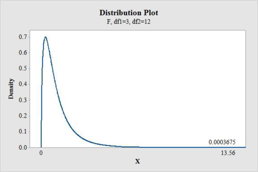
Conclusion:

The P-value for the F-statistic is 0.00037 and the level of significance is 0.01.

The P-value is less than the level of significance.

That is, $0.00037\left(=\text{P-value}\right)<0.01\left(=\alpha \right)$.

Thus, there is strong evidence to conclude that the mean number of unpopped kernels is different for at least one of the four brands of popcorn.

d.

To determine

Suggest what else about the data would be useful to check the assumptions and conditions.

Explanation of Solution

The side by side boxplot of the treatments would be useful to check the similar variance conditions and also the spread of the data.

The normal probability of residuals can be used to check the normality assumption of the error term. If the points in the normal probability plot lies approximately on a straight line it assumed that the residuals are normally distributed.

Also, residual plot is used to identify pattern and spread of the residuals.