Chapter 25, Problem 14E

To determine

(a)

To compute:

The profit-maximizing quantity and price for the monopolist if marginal cost is constant at $4 at all levels of output.

Answer to Problem 14E

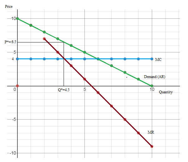
The profit-maximizing quantity and price are Q*=4.5 and P*=$6.5.

Explanation of Solution

The price and quantity schedule is given. The profit-maximizing output for a monopoly is given by the following condition:

  $\begin{array}{l}\text{Profit-maximizing}\text{conditon:}\\ \boxed{\text{MR=MC}}\end{array}$

The marginal cost is constant at $4 for all levels of output. The total proceeds or income from sale of a given level of output is called total revenue (TR). While the additional revenue generated from sale of an additional level of output is regarded a marginal revenue (MR).

First, calculate TR and MR using the formula below.

  $\begin{array}{l}\text{TR=P×Q}\\ {\text{MR}}_{\text{n}}{\text{=TR}}_{\text{n}}{\text{-TR}}_{\text{n-1}}\end{array}$

Price (P)	Output (Q)	TR (Total Revenue)	MR (Marginal Revenue)	MC (Marginal Cost)
10	0	0	0	4
9	1	9	9	4
8	2	16	7	4
7	3	21	5	4
6	4	24	3	4
5	5	25	1	4
4	6	24	-1	4
3	7	21	-3	4
2	8	16	-5	4
1	9	9	-7	4
0	10	0	-9	4

Using the MR and MC schedules in the table above, draw the graph for MR and MC. The profit-maximizing quantity and price are Q*=4.5 and P*=$6.5.

Economics Concept Introduction

Monopoly:

Monopoly is a market structure where only one seller exists, and product is differentiated.

Demand:

The demand for a good is the quantity of that good that consumers are willing and able to purchase at different prices.

Total Revenue (TR):

The total proceeds or income from sale of a given level of output is called total revenue.

Marginal Revenue (MR):

The additional revenue generated from sale of an additional level of output is regarded a marginal revenue.

Average Revenue (AR):

When at any level of output, the total revenue is divided by that level of output, we get the average revenue. AR is also the demand curve.

Total cost (TC):

The total outlay in production activity is referred to as total cost.

Marginal Cost (MC):

The additional cost of producing an extra unit of output is referred to as the marginal cost of producing that unit of output.

To determine

(b)

To compute:

The deadweight loss from the output choice of monopolist vis-à-vis perfect competition.

Answer to Problem 14E

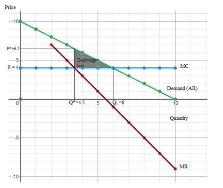
The deadweight loss resulting from the production of monopoly output is $1.875.

Explanation of Solution

Perfect competition is a market structure where large number of buyers and sellers exist, and products are homogeneous. Monopoly is a market structure where only one seller exists, and product is differentiated.

The case of perfect competition is regarded as the benchmark case since the output produced is socially optimum where there is full utilization of resources and no underemployment exists. It implies that the competitive output is such that allocative efficiency is achieved. Resultantly, there is no loss in social surplus and no deadweight loss. The equilibrium output in case of perfect competition is given by the condition P=MC and is indicated as Q_c in the diagram below.

Under monopoly, the monopolist produces where MR=MC. Monopoly results in deadweight loss since the output produced is less than socially optimum output.

The deadweight loss in case of monopoly is calculated and shown below:

  $\begin{array}{c}\text{Deadweight}\text{loss}=\text{Area}\text{of}\text{shaded}\text{triangle}\\ =\frac{\text{1}}{\text{2}}\text{×(6}-\text{4}\text{.5)}\times \text{(\$6}\text{.5}-\text{\$4)}\\ =\text{\$1}\text{.875}\end{array}$

Economics Concept Introduction

Perfect competition:

It is a market structure where large number of buyers and sellers exist, and products are homogeneous.

Monopoly:

Monopoly is a market structure where only one seller exists, and product is differentiated.

Deadweight loss:

It is the loss in social surplus that is due to production of less than socially optimum output.

Demand:

The demand for a good is the quantity of that good that consumers are willing and able to purchase at different prices.

Total Revenue (TR):

The total proceeds or income from sale of a given level of output is called total revenue.

Marginal Revenue (MR):

The additional revenue generated from sale of an additional level of output is regarded a marginal revenue.

Average Revenue (AR):

When at any level of output, the total revenue is divided by that level of output, we get the average revenue. AR is also the demand curve.

Total cost (TC):

The total outlay in production activity is referred to as total cost.

Marginal Cost (MC):

The additional cost of producing an extra unit of output is referred to as the marginal cost of producing that unit of output.