
Videos
(a)
To construct: The stemplot for Diabetic Mice and Normal Mice.
To check: Whether it appears that potentials in the two groups differ in a systematic way or not.
(a)
Answer to Problem 24.58SE
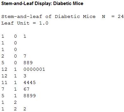
Stemplot for Diabetic Mice:
Output using the MINITAB software is given below:
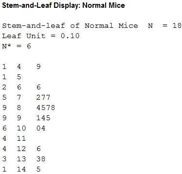
Stemplot for Normal Mice:
Output using the MINITAB software is given below:
Yes, it appears that potentials in the two groups differ in a systematic way.
Explanation of Solution
Given info:
The data shows the measured the difference in electrical potential between the Diabetic Mice and Normal Mice.
Calculation:
Stemplot for Diabetic Mice:
Software procedure:
Step by step procedure to construct Stemplot for Diabetic Mice by using the MINITAB software:
- Choose Graph > Stem-and-Leaf.
- In Graph variables, enter the column of Diabetic Mice.
- Click OK.
Observation:
From Stemplot for Diabetic Mice, it is clear that the left side of the stemplot extended larger than the right side of the stemplot. Hence, the distribution of the Diabetic Mice is left-skewed with one low outlier.
Stemplot for Normal Mice:
Software procedure:
Step by step procedure to construct Stemplot for Normal Mice by using the MINITAB software:
- Choose Graph > Stem-and-Leaf.
- In Graph variables, enter the column of Normal Mice.
- Click OK.
Observation:
From Stemplot for Normal Mice, it is clear that the right side of the stemplot extended same as in the left side of the stemplot. Hence, the distribution of the Normal Mice is symmetric.
Justification:
From the Stemplot for Diabetic Mice and Normal Mice, it can be observed that the distribution of the two groups is symmetric without considering the outliers. Hence, it appears that potentials in the two groups differ in a systematic way.
(b)
To test: Whether there is a significant difference in
(b)
Answer to Problem 24.58SE
The conclusion is that, there is a significant difference in mean potentials between the two groups.
Explanation of Solution
Calculation:
PLAN:
Check whether or not there is a significant difference in mean potentials between the two groups.
State the test hypotheses.
Null hypothesis:
Alternative hypothesis:
SOLVE:
Test statistic and P-value:
Software procedure:
Step by step procedure to obtain test statistic and P-value using the MINITAB software:
- Choose Stat > Basic Statistics > 2-Sample t.
- Choose Sample in different columns.
- In First, enter the column of Diabetic Mice.
- In Second, enter the column of Normal Mice.
- Choose Options.
- In Confidence level, enter 95.
- In Alternative, select not equal.
- Click OK in all the dialogue boxes.
Output using the MINITAB software is given below:
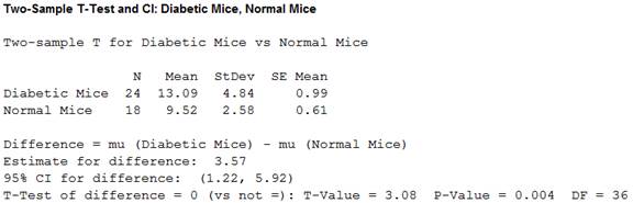
From the MINITAB output, the value of the t-statistic is 3.08 and the P-value is 0.004.
CONCLUDE:
The P-value is 0.004 and the significance level is 0.05.
Here, the P-value is less than the significance level.
That is,
Therefore, by the rejection rule, it can be concluded that there is evidence to reject
Thus, there is a significant difference in mean potentials between the two groups.
(c)
To test: Whether there is a significant difference in mean potentials between the two groups or not.
To check: Whether the outlier affects the conclusion or not.
(c)
Answer to Problem 24.58SE
The conclusion is that, there is a significant difference in mean potentials between the two groups.
No, the outlier does not affect the conclusion.
Explanation of Solution
Calculation:
PLAN:
Check whether or not there is a significant difference in mean potentials between the two groups.
State the test hypotheses.
Null hypothesis:
Alternative hypothesis:
SOLVE:
Test statistic and P-value:
Software procedure:
Step by step procedure to obtain test statistic and P-value without outlier using the MINITAB software:
- Choose Stat > Basic Statistics > 2-Sample t.
- Choose Sample in different columns.
- In First, enter the column of Diabetic Mice.
- In Second, enter the column of Normal Mice.
- Choose Options.
- In Confidence level, enter 95.
- In Alternative, select not equal.
- Click OK in all the dialogue boxes.
Output using the MINITAB software is given below:
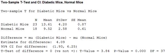
From the MINITAB output, the value of the t-statistic is 3.84 and the P-value is 0.000.
CONCLUDE:
The P-value is 0.000 and the significance level is 0.05.
Here, the P-value is less than the significance level.
That is,
Therefore, by the rejection rule, it can be concluded that there is evidence to reject
Thus, there is a significant difference in mean potentials between the two groups.
Justification:
From the results, it can be observed that the conclusions for inference with outlier and without outlier are same. Hence, the outlier does not affect the conclusion.
Want to see more full solutions like this?
Chapter 24 Solutions
BASIC PRACTICE OF STATS-LL W/SAPLINGPLU


- Using the method of sections need help solving this please explain im stuckarrow_forwardPlease solve 6.31 by using the method of sections im stuck and need explanationarrow_forwarda) When two variables are correlated, can the researcher be sure that one variable causes the other? If YES , why? If NO , why? b) What is meant by the statement that two variables are related? Discuss.arrow_forward
- SCIE 211 Lab 3: Graphing and DataWorksheetPre-lab Questions:1. When should you use each of the following types of graphs? Fill answers in the table below.Type of Graph Used to showLine graphScatter plotBar graphHistogramPie Chart2. Several ways in which we can be fooled or misled by a graph were identified in the Lab 3Introduction. Find two examples of misleading graphs on the Internet and paste them below. Besure to identify why each graph is misleading. Data Charts:Circumference vs. Diameter for circular objectsDiameter Can 1 (cm) Can 2 (cm) Can 3 (cm)Trial 1Trial 2Trial 3MeanCircumference Can 1 (cm) Can 2 (cm) Can 3 (cm)Trial 1Trial 2Trial 3MeanScatter Plot Graph – Circumference Vs. DiameterIdentify 2 points of the Trendline.Y1 = ________ Y2 = _________X1 = ________ X2 = _________Calculate the Slope of the Trendline = Post-lab Questions:1. Answer the questions below. You will need to use the following equation to answer…arrow_forwardThe U.S. Bureau of Labor Statistics reports that 11.3% of U.S. workers belong to unions (BLS website, January 2014). Suppose a sample of 400 U.S. workers is collected in 2014 to determine whether union efforts to organize have increased union membership. a. Formulate the hypotheses that can be used to determine whether union membership increased in 2014.H 0: p H a: p b. If the sample results show that 52 of the workers belonged to unions, what is the p-value for your hypothesis test (to 4 decimals)?arrow_forwardA company manages an electronic equipment store and has ordered 200200 LCD TVs for a special sale. The list price for each TV is $200200 with a trade discount series of 6 divided by 10 divided by 2.6/10/2. Find the net price of the order by using the net decimal equivalent.arrow_forward
- According to flightstats.com, American Airlines flights from Dallas to Chicago are on time 80% of the time. Suppose 10 flights are randomly selected, and the number of on-time flights is recorded. (a) Explain why this is a binomial experiment. (b) Determine the values of n and p. (c) Find and interpret the probability that exactly 6 flights are on time. (d) Find and interpret the probability that fewer than 6 flights are on time. (e) Find and interpret the probability that at least 6 flights are on time. (f) Find and interpret the probability that between 4 and 6 flights, inclusive, are on time.arrow_forwardShow how you get critical values of 1.65, -1.65, and $1.96 for a right-tailed, left- tailed, and two-tailed hypothesis test (use a = 0.05 and assume a large sample size).arrow_forwardSuppose that a sports reporter claims the average football game lasts 3 hours, and you believe it's more than that. Your random sample of 35 games has an average time of 3.25 hours. Assume that the population standard deviation is 1 hour. Use a = 0.05. What do you conclude?arrow_forward
- Suppose that a pizza place claims its average pizza delivery time is 30 minutes, but you believe it takes longer than that. Your sample of 10 pizzas has an average delivery time of 40 minutes. Assume that the population standard deviation is 15 minutes and the times have a normal distribution. Use a = 0.05. a. What are your null and alternative hypotheses? b. What is the critical value? c. What is the test statistic? d. What is the conclusion?arrow_forwardTable 5: Measurement Data for Question 9 Part Number Op-1, M-1 Op-1, M-2 | Op-2, M-1 Op-2, M-2 | Op-3, M-1 Op-3, M-2 1 21 20 20 20 19 21 2 24 23 24 24 23 24 3 4 5 6 7 8 9 10 11 21 12 8222332 201 21 20 22 20 22 27 27 28 26 27 28 19 18 19 21 24 21 22 19 17 18 24 23 25 25 23 26 20 20 18 19 17 13 23 25 25 2 3 3 3 3 2 3 18 18 21 21 23 22 24 22 20 19 23 24 25 24 20 21 19 18 25 25 14 24 24 23 25 24 15 29 30 30 28 31 16 26 26 25 26 25 17 20 20 19 20 20 843882388 20 18 25 20 19 25 25 30 27 20 18 19 21 19 19 21 23 19 25 26 25 24 25 25 20 19 19 18 17 19 17 Question 9 A measurement systems experiment involving 20 parts, three operators (Op-1, Op-2, Op-3), and two measure- ments (M-1, M-2) per part is shown in Table 5. (a) Estimate the repeatability and reproducibility of the gauge. (b) What is the estimate of total gauge variability?" (c) If the product specifications are at LSL = 6 and USL 60, what can you say about gauge capability?arrow_forwardQuestion 5 A fraction nonconforming control chart with center line 0.10, UCL = 0.19, and LCL = 0.01 is used to control a process. (a) If three-sigma limits are used, find the sample size for the control charte 2 (b) Use the Poisson approximation to the binomial to find the probability of type I error. (c) Use the Poisson approximation to the binomial to find the probability of type II error if the process fraction defective is actually p = 0.20.arrow_forward
 MATLAB: An Introduction with ApplicationsStatisticsISBN:9781119256830Author:Amos GilatPublisher:John Wiley & Sons Inc
 Probability and Statistics for Engineering and th...StatisticsISBN:9781305251809Author:Jay L. DevorePublisher:Cengage Learning
 Statistics for The Behavioral Sciences (MindTap C...StatisticsISBN:9781305504912Author:Frederick J Gravetter, Larry B. WallnauPublisher:Cengage Learning
 Elementary Statistics: Picturing the World (7th E...StatisticsISBN:9780134683416Author:Ron Larson, Betsy FarberPublisher:PEARSON
 The Basic Practice of StatisticsStatisticsISBN:9781319042578Author:David S. Moore, William I. Notz, Michael A. FlignerPublisher:W. H. Freeman
 Introduction to the Practice of StatisticsStatisticsISBN:9781319013387Author:David S. Moore, George P. McCabe, Bruce A. CraigPublisher:W. H. Freeman