
EFSC STA 2023 MML ACCESS
6th Edition
ISBN: 9780135927885
Author: Triola
Publisher: PEARSON
expand_more
expand_more
format_list_bulleted
Videos
Textbook Question
Chapter 2.3, Problem 10BSC
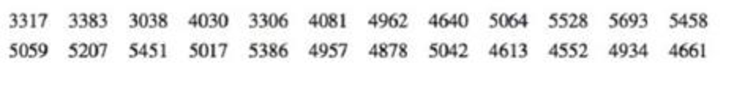
Time-Series Graphs. In Exercises 9 and 10, construct the time-series graph.
10. Home Runs Listed below are the numbers of home runs in Major League Baseball for each year beginning with 1990 (listed in order by row). Is there a trend?
Expert Solution & Answer
Want to see the full answer?
Check out a sample textbook solution
Students have asked these similar questions
A biologist is investigating the effect of potential plant
hormones by treating 20 stem segments. At the end of
the observation period he computes the following length
averages:
Compound X = 1.18
Compound Y = 1.17
Based on these mean values he concludes that there are
no treatment differences.
1) Are you satisfied with his conclusion? Why or why
not?
2) If he asked you for help in analyzing these data, what
statistical method would you suggest that he use to
come to a meaningful conclusion about his data and
why?
3) Are there any other questions you would ask him
regarding his experiment, data collection, and analysis
methods?
Business
What is the solution and answer to question?
Chapter 2 Solutions
EFSC STA 2023 MML ACCESS
Ch. 2.1 - McDonalds Dinner Service Times Refer 10 the...Ch. 2.1 - McDonalds Dinner Service Times Refer to the...Ch. 2.1 - Relative Frequency Distribution Use percentages to...Ch. 2.1 - Whats Wrong? Heights of adult males are known to...Ch. 2.1 - In Exercise 58, identify the class width, class...Ch. 2.1 - In Exercises 58, identify the class width, class...Ch. 2.1 - In Exercises 58, identify the class width, class...Ch. 2.1 - In Exercises 58, identify the class width, class...Ch. 2.1 - Normal Distributions. In Exercises 9 and 10, using...Ch. 2.1 - Normal Distributions. In Exercises 9 and 10, using...
Ch. 2.1 - Constructing Frequency Distributions. In Exercises...Ch. 2.1 - Constructing Frequency Distributions. In Exercises...Ch. 2.1 - Constructing Frequency Distributions. In Exercises...Ch. 2.1 - Burger King Dinner Service Times Refer to Data Set...Ch. 2.1 - Wendys Lunch Service Times Refer to Data Set 25...Ch. 2.1 - Wendys Dinner Service Times Refer to Data Set 25...Ch. 2.1 - Analysis of Last Digits Heights of statistics...Ch. 2.1 - Analysis of Last Digits Weights of respondents...Ch. 2.1 - Oscar Winners Construct one table (similar to...Ch. 2.1 - Blood Platelet Counts Construct one table (similar...Ch. 2.1 - Cumulative Frequency Distributions. In Exercises...Ch. 2.1 - Cumulative Frequency Distributions. In Exercises...Ch. 2.1 - Categorical Data. In Exercises 23 and 24, use the...Ch. 2.1 - Categorical Data. In Exercises 23 and 24, use the...Ch. 2.2 - Heights Heights of adult males are normally...Ch. 2.2 - More Heights The population of heights of adult...Ch. 2.2 - Blood Platelet Counts Listed below are blood...Ch. 2.2 - Blood Platelet Counts If we collect a sample of...Ch. 2.2 - Interpreting a Histogram. In Exercises 58, answer...Ch. 2.2 - Prob. 6BSCCh. 2.2 - Interpreting a Histogram. In Exercises 58, answer...Ch. 2.2 - Prob. 8BSCCh. 2.2 - Constructing Histograms. In Exercises 9-16,...Ch. 2.2 - Constructing Histograms. In Exercises 9-16,...Ch. 2.2 - Burger King Lunch Service Times Use the frequency...Ch. 2.2 - Burger King Dinner Service Times Use the frequency...Ch. 2.2 - Wendys Lunch Service Times Use the frequency...Ch. 2.2 - Wendys Dinner Service Times Use the frequency...Ch. 2.2 - Analysis of Last Digits Use the frequency...Ch. 2.2 - Analysis of Last Digits Use the frequency...Ch. 2.2 - Back-to-Back Relative Frequency Histograms When...Ch. 2.2 - Interpreting Normal Quantile Plots Which of the...Ch. 2.3 - Body Temperatures Listed below are body...Ch. 2.3 - Voluntary Response Data If we have a large...Ch. 2.3 - Ethics There are data showing that smoking is...Ch. 2.3 - CVDOT Section 2-1 introduced important...Ch. 2.3 - Dotplots. In Exercises 5 and 6, construct the...Ch. 2.3 - Diastolic Blood Pressure Listed below are...Ch. 2.3 - Stem plots. In Exercises 7 and 8, construct the...Ch. 2.3 - Stemplots. In Exercises 7 and 8, construct the...Ch. 2.3 - Time-Series Graphs. In Exercises 9 and 10,...Ch. 2.3 - Time-Series Graphs. In Exercises 9 and 10,...Ch. 2.3 - Pareto Charts. In Exercises 11 and 12 construct...Ch. 2.3 - Pareto Charts. In Exercises 11 and 12 construct...Ch. 2.3 - Pie Charts. In Exercises 13 and 14, construct the...Ch. 2.3 - Pie Charts. In Exercises 13 and 14, construct the...Ch. 2.3 - Frequency Polygon. In Exercises 15 and 16,...Ch. 2.3 - Frequency Polygon. In Exercises 15 and 16,...Ch. 2.3 - Self-Driving Vehicles In a survey of adults,...Ch. 2.3 - Deceptive Graphs. In Exercises 17-20, identify how...Ch. 2.3 - Deceptive Graphs. In Exercises 17-20, identify how...Ch. 2.3 - Deceptive Graphs. In Exercises 17-20, identify how...Ch. 2.3 - Expanded Stemplots A stemplot can be condensed by...Ch. 2.4 - Linear Correlation In this section we use r to...Ch. 2.4 - Causation A study has shown that there is a...Ch. 2.4 - Scanerplot What is a scatterplot and how does it...Ch. 2.4 - Estimating r For each of the following, estimate...Ch. 2.4 - Scatterplot. In Exercises 5-8, use the sample data...Ch. 2.4 - Scatterplot. In Exercises 5-8, use the sample data...Ch. 2.4 - Scatterplot. In Exercises 5-8, use the sample data...Ch. 2.4 - Scatterplot. In Exercises 5-8, use the sample data...Ch. 2.4 - Linear Correlation Coefficient In Exercises 9-12,...Ch. 2.4 - Linear Correlation Coefficient In Exercises 9-12,...Ch. 2.4 - Linear Correlation Coefficient In Exercises 9-12,...Ch. 2.4 - Using the data from Exercise 8 Heights of Fathers...Ch. 2.4 - Prob. 13BBCh. 2.4 - P-Values In Exercises 13-16, write a statement...Ch. 2.4 - P-Values In Exercises 13-16, write a statement...Ch. 2.4 - P-Values In Exercises 13-16, write a statement...Ch. 2 - Cookies Refer to the accompanying frequency...Ch. 2 - Cookies Using the same frequency distribution from...Ch. 2 - Cookies Using the same frequency distribution from...Ch. 2 - Cookies A stemplot of the same cookies summarized...Ch. 2 - Computers As a quality control manager at Texas...Ch. 2 - Distribution of Wealth In recent years, there has...Ch. 2 - Health Test In an investigation of a relationship...Ch. 2 - Lottery In Floridas Play 4 lottery game, four...Ch. 2 - Seatbelts The Beams Seatbelts company...Ch. 2 - Seatbelts A histogram is to be constructed from...Ch. 2 - Frequency Distribution of Body Temperatures...Ch. 2 - Histogram of Body Temperatures Construct the...Ch. 2 - Dotplot of Body Temperatures Construct a dotplot...Ch. 2 - Stemplot of Body Temperatures Construct a stemplot...Ch. 2 - Body Temperatures Listed below are the...Ch. 2 - Environment a. After collecting the average (mean)...Ch. 2 - Its Like Time Do This Exercise In a Marist survey...Ch. 2 - Whatever Use the same data from Exercise 7 to...Ch. 2 - In Exercises 1-6 refer to the data below, which...Ch. 2 - Frequency Distribution For the frequency...Ch. 2 - In Exercises 1-6, refer to the data below, which...Ch. 2 - In Exercises 1-6, refer to the data below, which...Ch. 2 - In Exercises 1-6, refer to the data below, which...Ch. 2 - Data Type a. The listed playing times are all...
Knowledge Booster


Learn more about
Need a deep-dive on the concept behind this application? Look no further. Learn more about this topic, statistics and related others by exploring similar questions and additional content below.Similar questions
- To: [Boss's Name] From: Nathaniel D Sain Date: 4/5/2025 Subject: Decision Analysis for Business Scenario Introduction to the Business Scenario Our delivery services business has been experiencing steady growth, leading to an increased demand for faster and more efficient deliveries. To meet this demand, we must decide on the best strategy to expand our fleet. The three possible alternatives under consideration are purchasing new delivery vehicles, leasing vehicles, or partnering with third-party drivers. The decision must account for various external factors, including fuel price fluctuations, demand stability, and competition growth, which we categorize as the states of nature. Each alternative presents unique advantages and challenges, and our goal is to select the most viable option using a structured decision-making approach. Alternatives and States of Nature The three alternatives for fleet expansion were chosen based on their cost implications, operational efficiency, and…arrow_forwardBusinessarrow_forwardWhy researchers are interested in describing measures of the center and measures of variation of a data set?arrow_forward
- WHAT IS THE SOLUTION?arrow_forwardThe following ordered data list shows the data speeds for cell phones used by a telephone company at an airport: A. Calculate the Measures of Central Tendency from the ungrouped data list. B. Group the data in an appropriate frequency table. C. Calculate the Measures of Central Tendency using the table in point B. 0.8 1.4 1.8 1.9 3.2 3.6 4.5 4.5 4.6 6.2 6.5 7.7 7.9 9.9 10.2 10.3 10.9 11.1 11.1 11.6 11.8 12.0 13.1 13.5 13.7 14.1 14.2 14.7 15.0 15.1 15.5 15.8 16.0 17.5 18.2 20.2 21.1 21.5 22.2 22.4 23.1 24.5 25.7 28.5 34.6 38.5 43.0 55.6 71.3 77.8arrow_forwardII Consider the following data matrix X: X1 X2 0.5 0.4 0.2 0.5 0.5 0.5 10.3 10 10.1 10.4 10.1 10.5 What will the resulting clusters be when using the k-Means method with k = 2. In your own words, explain why this result is indeed expected, i.e. why this clustering minimises the ESS map.arrow_forward
- why the answer is 3 and 10?arrow_forwardPS 9 Two films are shown on screen A and screen B at a cinema each evening. The numbers of people viewing the films on 12 consecutive evenings are shown in the back-to-back stem-and-leaf diagram. Screen A (12) Screen B (12) 8 037 34 7 6 4 0 534 74 1645678 92 71689 Key: 116|4 represents 61 viewers for A and 64 viewers for B A second stem-and-leaf diagram (with rows of the same width as the previous diagram) is drawn showing the total number of people viewing films at the cinema on each of these 12 evenings. Find the least and greatest possible number of rows that this second diagram could have. TIP On the evening when 30 people viewed films on screen A, there could have been as few as 37 or as many as 79 people viewing films on screen B.arrow_forwardQ.2.4 There are twelve (12) teams participating in a pub quiz. What is the probability of correctly predicting the top three teams at the end of the competition, in the correct order? Give your final answer as a fraction in its simplest form.arrow_forward
- The table below indicates the number of years of experience of a sample of employees who work on a particular production line and the corresponding number of units of a good that each employee produced last month. Years of Experience (x) Number of Goods (y) 11 63 5 57 1 48 4 54 5 45 3 51 Q.1.1 By completing the table below and then applying the relevant formulae, determine the line of best fit for this bivariate data set. Do NOT change the units for the variables. X y X2 xy Ex= Ey= EX2 EXY= Q.1.2 Estimate the number of units of the good that would have been produced last month by an employee with 8 years of experience. Q.1.3 Using your calculator, determine the coefficient of correlation for the data set. Interpret your answer. Q.1.4 Compute the coefficient of determination for the data set. Interpret your answer.arrow_forwardCan you answer this question for mearrow_forwardTechniques QUAT6221 2025 PT B... TM Tabudi Maphoru Activities Assessments Class Progress lIE Library • Help v The table below shows the prices (R) and quantities (kg) of rice, meat and potatoes items bought during 2013 and 2014: 2013 2014 P1Qo PoQo Q1Po P1Q1 Price Ро Quantity Qo Price P1 Quantity Q1 Rice 7 80 6 70 480 560 490 420 Meat 30 50 35 60 1 750 1 500 1 800 2 100 Potatoes 3 100 3 100 300 300 300 300 TOTAL 40 230 44 230 2 530 2 360 2 590 2 820 Instructions: 1 Corall dawn to tha bottom of thir ceraan urina se se tha haca nariad in archerca antarand cubmit Q Search ENG US 口X 2025/05arrow_forward
arrow_back_ios
SEE MORE QUESTIONS
arrow_forward_ios
Recommended textbooks for you
 Glencoe Algebra 1, Student Edition, 9780079039897...AlgebraISBN:9780079039897Author:CarterPublisher:McGraw Hill
 Holt Mcdougal Larson Pre-algebra: Student Edition...AlgebraISBN:9780547587776Author:HOLT MCDOUGALPublisher:HOLT MCDOUGAL
 Big Ideas Math A Bridge To Success Algebra 1: Stu...AlgebraISBN:9781680331141Author:HOUGHTON MIFFLIN HARCOURTPublisher:Houghton Mifflin Harcourt
 Trigonometry (MindTap Course List)TrigonometryISBN:9781305652224Author:Charles P. McKeague, Mark D. TurnerPublisher:Cengage Learning
Glencoe Algebra 1, Student Edition, 9780079039897...
Algebra
ISBN:9780079039897
Author:Carter
Publisher:McGraw Hill
Holt Mcdougal Larson Pre-algebra: Student Edition...
Algebra
ISBN:9780547587776
Author:HOLT MCDOUGAL
Publisher:HOLT MCDOUGAL
Big Ideas Math A Bridge To Success Algebra 1: Stu...
Algebra
ISBN:9781680331141
Author:HOUGHTON MIFFLIN HARCOURT
Publisher:Houghton Mifflin Harcourt
Trigonometry (MindTap Course List)
Trigonometry
ISBN:9781305652224
Author:Charles P. McKeague, Mark D. Turner
Publisher:Cengage Learning
Time Series Analysis Theory & Uni-variate Forecasting Techniques; Author: Analytics University;https://www.youtube.com/watch?v=_X5q9FYLGxM;License: Standard YouTube License, CC-BY
Operations management 101: Time-series, forecasting introduction; Author: Brandoz Foltz;https://www.youtube.com/watch?v=EaqZP36ool8;License: Standard YouTube License, CC-BY