
Videos
Protein Grams in Fast Food The amount of protein (in grams) for a variety of fast-food sandwiches is reported here. Construct a frequency distribution, using 6 classes. Draw a histogram, a frequency
To Sketch: A histogram, frequency polygon and ogive using relative frequency and describe the shape of the histogram for the given data.
Answer to Problem 18E
The sketches of all three graphs are as follows:
The shape of the histogram is right skewed.
Explanation of Solution
Given Info:
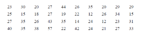
The amount of protein (in grams) for a variety of fast-food sandwiches is reported here
| 23 | 30 | 20 | 27 | 44 | 26 | 35 | 20 | 29 | 29 |
| 25 | 15 | 18 | 27 | 19 | 22 | 12 | 26 | 34 | 15 |
| 27 | 35 | 26 | 43 | 35 | 14 | 24 | 12 | 23 | 31 |
| 40 | 35 | 38 | 57 | 22 | 42 | 24 | 21 | 27 | 33 |
Calculation:
The class boundaries for any class are given by:
The grouped frequency distribution is as follows:
| Class limit | Class boundaries |  Tally Tally |
Frequency |
| 12-19 | 11.5-19.5 |  |
7 |
| 20-27 | 19.5-27.5 |  |
17 |
| 28-35 | 27.5-35.5 | 10 | |
| 36-43 | 35.5-43.5 |
|
4 |
| 44-51 | 43.5-51.5 |
|
1 |
| 52-59 | 51.5-59.5 |
|
1 |
Class midpoint:
The midpoint of class boundaries is obtained by adding lower and upper limit and dividing by 2.
For the first class,
Thus, the midpoint for the first class is 22.
Similarly, the midpoint for other classes was obtained.
Relative frequency distribution:
The relative frequency is the ration of a class frequency to the total frequency. Cumulative relative frequency can also defined as the sum of all previous frequencies up to the current point.
| Class boundaries | Frequency | Mid point |
Relative frequency |
Cumulative relative frequency |
| 11.5-19.5 | 7 | 15.5 | 0.175 | 0.175 |
| 19.5-27.5 | 17 | 23.5 | 0.425 | 0.6 |
| 27.5-35.5 | 10 | 31.5 | 0.25 | 0.85 |
| 35.5-43.5 | 4 | 39.5 | 0.1 | 0.95 |
| 43.5-51.5 | 1 | 47.5 | 0.025 | 0.975 |
| 51.5-59.5 | 1 | 55.5 | 0.025 | 1 |
| Total | 40 |
The histogram is a graph that displays the data by using contiguous vertical bars of various heights to represent the frequencies of the classes.
| Upper limit | Relative frequency |
| 19.5 | 0.175 |
| 27.5 | 0.425 |
| 35.5 | 0.25 |
| 43.5 | 0.1 |
| 51.5 | 0.025 |
| 59.5 | 0.025 |
Histogram:
Software procedure:
Step by step procedure for constructing histogram using Excel is given below:
- Press [Ctrl]-N for a new workbook.
- Enter the data in column A, one number per cell.
- Enter the upper boundaries into column B.
- From the toolbar, select the Data tab, then select Data Analysis.
- In Data Analysis, select Histogram and click [OK].
- In the Histogram dialog box, select relative column in the Input Range box and select upper limit column in the Bin Range box.
- Select New Worksheet Ply and Chart Output. Click [OK].
Output obtained from Excel is given below:
Shape of the distribution:
Symmetric:
A distribution is said to be symmetric if the left side of histogram is the mirror image of the right side of histogram.
Skewed right:
If the right side of the distribution extends far away than the left side of histogram, it is said to be skewed right.
Skewed left:
If the left side of the distribution extends far away than the right side of histogram, it is said to be skewed left.
Here, the histogram extends far away than the left side of histogram, it is said to be skewed right.
Hence, the distribution for the amount of protein (in grams) for a variety of fast-food sandwiches is skewed right.
Frequency polygons:
Step by step procedure for constructing frequency polygon using Excel is given below:
- Press [CTRL]-N for a new notebook.
- Enter the midpoints of the data into column A and the frequencies into column B including labels.
- Press and hold the left mouse button, and drag over the Frequencies (including the label) from column B.
- Select the Insert tab from the toolbar and the Line Chart option.
- Select the 2-D line chart type.
Output obtained from Excel is given below:

Frequency ogive:
Step by step procedure for constructing frequency ogive using Excel is given below:
- To create an ogive, use the upper class boundaries (horizontal axis) and cumulative frequencies (vertical axis) from the frequency distribution.
- Type the upper class boundaries (including a class with frequency 0 before the lowest class to anchor the graph to the horizontal axis) and
- Corresponding cumulative frequencies into adjacent columns of an Excel worksheet.
- Press and hold the left mouse button, and drag over the Cumulative Frequencies from column B.
- Select Line Chart, then the 2-D Line option.
Output obtained from Excel is given below:

The points plotted are the upper class limit and the corresponding cumulative relative frequency.
Want to see more full solutions like this?
Chapter 2 Solutions
ELEMENTARY STATISTICS: STEP BY STEP- ALE


- The U.S. Postal Service will ship a Priority Mail® Large Flat Rate Box (12" 3 12" 3 5½") any where in the United States for a fixed price, regardless of weight. The weights (ounces) of 20 ran domly chosen boxes are shown below. (a) Make a stem-and-leaf diagram. (b) Make a histogram. (c) Describe the shape of the distribution. Weights 72 86 28 67 64 65 45 86 31 32 39 92 90 91 84 62 80 74 63 86arrow_forward(a) What is a bimodal histogram? (b) Explain the difference between left-skewed, symmetric, and right-skewed histograms. (c) What is an outlierarrow_forward(a) Test the hypothesis. Consider the hypothesis test Ho = : against H₁o < 02. Suppose that the sample sizes aren₁ = 7 and n₂ = 13 and that $² = 22.4 and $22 = 28.2. Use α = 0.05. Ho is not ✓ rejected. 9-9 IV (b) Find a 95% confidence interval on of 102. Round your answer to two decimal places (e.g. 98.76).arrow_forward
- Let us suppose we have some article reported on a study of potential sources of injury to equine veterinarians conducted at a university veterinary hospital. Forces on the hand were measured for several common activities that veterinarians engage in when examining or treating horses. We will consider the forces on the hands for two tasks, lifting and using ultrasound. Assume that both sample sizes are 6, the sample mean force for lifting was 6.2 pounds with standard deviation 1.5 pounds, and the sample mean force for using ultrasound was 6.4 pounds with standard deviation 0.3 pounds. Assume that the standard deviations are known. Suppose that you wanted to detect a true difference in mean force of 0.25 pounds on the hands for these two activities. Under the null hypothesis, 40 = 0. What level of type II error would you recommend here? Round your answer to four decimal places (e.g. 98.7654). Use a = 0.05. β = i What sample size would be required? Assume the sample sizes are to be equal.…arrow_forward= Consider the hypothesis test Ho: μ₁ = μ₂ against H₁ μ₁ μ2. Suppose that sample sizes are n₁ = 15 and n₂ = 15, that x1 = 4.7 and X2 = 7.8 and that s² = 4 and s² = 6.26. Assume that o and that the data are drawn from normal distributions. Use απ 0.05. (a) Test the hypothesis and find the P-value. (b) What is the power of the test in part (a) for a true difference in means of 3? (c) Assuming equal sample sizes, what sample size should be used to obtain ẞ = 0.05 if the true difference in means is - 2? Assume that α = 0.05. (a) The null hypothesis is 98.7654). rejected. The P-value is 0.0008 (b) The power is 0.94 . Round your answer to four decimal places (e.g. Round your answer to two decimal places (e.g. 98.76). (c) n₁ = n2 = 1 . Round your answer to the nearest integer.arrow_forwardConsider the hypothesis test Ho: = 622 against H₁: 6 > 62. Suppose that the sample sizes are n₁ = 20 and n₂ = 8, and that = 4.5; s=2.3. Use a = 0.01. (a) Test the hypothesis. Round your answers to two decimal places (e.g. 98.76). The test statistic is fo = i The critical value is f = Conclusion: i the null hypothesis at a = 0.01. (b) Construct the confidence interval on 02/022 which can be used to test the hypothesis: (Round your answer to two decimal places (e.g. 98.76).) iarrow_forward
- 2011 listing by carmax of the ages and prices of various corollas in a ceratin regionarrow_forwardس 11/ أ . اذا كانت 1 + x) = 2 x 3 + 2 x 2 + x) هي متعددة حدود محسوبة باستخدام طريقة الفروقات المنتهية (finite differences) من جدول البيانات التالي للدالة (f(x . احسب قيمة . ( 2 درجة ) xi k=0 k=1 k=2 k=3 0 3 1 2 2 2 3 αarrow_forward1. Differentiate between discrete and continuous random variables, providing examples for each type. 2. Consider a discrete random variable representing the number of patients visiting a clinic each day. The probabilities for the number of visits are as follows: 0 visits: P(0) = 0.2 1 visit: P(1) = 0.3 2 visits: P(2) = 0.5 Using this information, calculate the expected value (mean) of the number of patient visits per day. Show all your workings clearly. Rubric to follow Definition of Random variables ( clearly and accurately differentiate between discrete and continuous random variables with appropriate examples for each) Identification of discrete random variable (correctly identifies "number of patient visits" as a discrete random variable and explains reasoning clearly.) Calculation of probabilities (uses the probabilities correctly in the calculation, showing all steps clearly and logically) Expected value calculation (calculate the expected value (mean)…arrow_forward
- if the b coloumn of a z table disappeared what would be used to determine b column probabilitiesarrow_forwardConstruct a model of population flow between metropolitan and nonmetropolitan areas of a given country, given that their respective populations in 2015 were 263 million and 45 million. The probabilities are given by the following matrix. (from) (to) metro nonmetro 0.99 0.02 metro 0.01 0.98 nonmetro Predict the population distributions of metropolitan and nonmetropolitan areas for the years 2016 through 2020 (in millions, to four decimal places). (Let x, through x5 represent the years 2016 through 2020, respectively.) x₁ = x2 X3 261.27 46.73 11 259.59 48.41 11 257.96 50.04 11 256.39 51.61 11 tarrow_forwardIf the average price of a new one family home is $246,300 with a standard deviation of $15,000 find the minimum and maximum prices of the houses that a contractor will build to satisfy 88% of the market valuearrow_forward
 Holt Mcdougal Larson Pre-algebra: Student Edition...AlgebraISBN:9780547587776Author:HOLT MCDOUGALPublisher:HOLT MCDOUGAL
 Big Ideas Math A Bridge To Success Algebra 1: Stu...AlgebraISBN:9781680331141Author:HOUGHTON MIFFLIN HARCOURTPublisher:Houghton Mifflin Harcourt
 Glencoe Algebra 1, Student Edition, 9780079039897...AlgebraISBN:9780079039897Author:CarterPublisher:McGraw Hill