Concept explainers
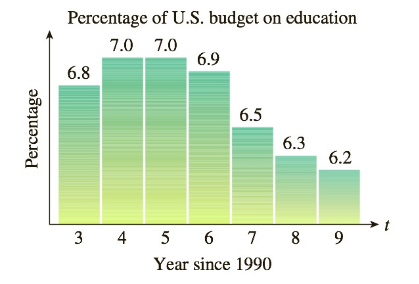
Education Expenditure The following chart shows the percentage of the U.S. discretionary budget allocated to education from 2003 to 2009. (

Source: www.globalissues.org/Geopolitics/ArmsTrade/Spending.asp
a. If you want to model the percentage figures with a function of the form
b. Which of the following models best approximates the data given? (Try to answer this without actually computing values.)
A.
B.
C.
D.
c. What is the nearest year that would correspond to the vertex of the graph of the correct model from part (b)? What is the danger of extrapolating the data in either direction?
Trending nowThis is a popular solution!

Chapter 2 Solutions
Applied Calculus
- For each graph in Figure 16, determine whether f (1) is larger or smaller than the slope of the secant line between x = 1 and x = 1 + h for h > 0. Explain your reasoningarrow_forwardPoints z1 and z2 are shown on the graph.z1 is at (4 real,6 imaginary), z2 is at (-5 real, 2 imaginary)Part A: Identify the points in standard form and find the distance between them.Part B: Give the complex conjugate of z2 and explain how to find it geometrically.Part C: Find z2 − z1 geometrically and explain your steps.arrow_forwardA polar curve is represented by the equation r1 = 7 + 4cos θ.Part A: What type of limaçon is this curve? Justify your answer using the constants in the equation.Part B: Is the curve symmetrical to the polar axis or the line θ = pi/2 Justify your answer algebraically.Part C: What are the two main differences between the graphs of r1 = 7 + 4cos θ and r2 = 4 + 4cos θ?arrow_forward
- A curve, described by x2 + y2 + 8x = 0, has a point A at (−4, 4) on the curve.Part A: What are the polar coordinates of A? Give an exact answer.Part B: What is the polar form of the equation? What type of polar curve is this?Part C: What is the directed distance when Ø = 5pi/6 Give an exact answer.arrow_forwardNew folder 10. Find the area enclosed by the loop of the curve (1- t², t-t³)arrow_forward1. Graph and find the corresponding Cartesian equation for: t X== y = t +1 2 te(-∞, ∞) 42,369 I APR 27 F5 3 MacBook Air stv A Aa T 4 DIIarrow_forward
- Middle School GP... Echo home (1) Addition and su... Google Docs Netflix Netflix New folder 9. Find the area enclosed by x = sin²t, y = cost and the y-axis.arrow_forward2. Graph and find the corresponding Cartesian equation for: (4 cos 0,9 sin 0) θ ε [0, 2π) 42,369 I APR 27 3 MacBook Air 2 tv A Aaarrow_forward30 Page< 3. Find the equation of the tangent line for x = 1+12, y = 1-3 at t = 2 42,369 APR A 27 M . tv NA 1 TAGN 2 Aa 7 MacBook Air #8arrow_forward
- Evaluate the following integrals as they are writtenarrow_forwardCalculus lll May I please have the blank lines completed, and final statement defined as a result? Thank you for the support!arrow_forward3. Consider the polynomial equation 6-iz+7z² - iz³ +z = 0 for which the roots are 3i, -2i, -i, and i. (a) Verify the relations between this roots and the coefficients of the polynomial. (b) Find the annulus region in which the roots lie.arrow_forward
 Glencoe Algebra 1, Student Edition, 9780079039897...AlgebraISBN:9780079039897Author:CarterPublisher:McGraw Hill
 Trigonometry (MindTap Course List)TrigonometryISBN:9781305652224Author:Charles P. McKeague, Mark D. TurnerPublisher:Cengage Learning
 Big Ideas Math A Bridge To Success Algebra 1: Stu...AlgebraISBN:9781680331141Author:HOUGHTON MIFFLIN HARCOURTPublisher:Houghton Mifflin Harcourt
 Trigonometry (MindTap Course List)TrigonometryISBN:9781337278461Author:Ron LarsonPublisher:Cengage Learning
 Functions and Change: A Modeling Approach to Coll...AlgebraISBN:9781337111348Author:Bruce Crauder, Benny Evans, Alan NoellPublisher:Cengage Learning


