Sub part (a):
Impact of different views on inflation on the economy's equilibrium.
Sub part (a):
Explanation of Solution
The supply is dependent upon the
The
When the new chairman is one with the view that the inflation is not a big issue on the economy, the economy would identify the chairman as the silent supporter of the inflation, and they will expect that the chairman will not introduce the active policies to fight against and control the inflation in the economy. As a result, the public will expect that the rise in the inflation and the price level are likely to rise.
Concept introduction:
Aggregate demand curve: It is the curve that shows the relationship between the price level in the economy and the quantity of real GDP demanded by the economic agents such as the households, firms, and the government.
Equilibrium: The equilibrium in the economy is the point where the economy's aggregate demand curve and the aggregate supply curve intersect with each other. There will be no excess demand or
Sub part (b):
Impact of different views on inflation on the economy's equilibrium.
Sub part (b):
Explanation of Solution
When the people expect higher inflation for the next year, they will start to calculate the changes in the price level. According to the expected higher level of inflation over the next year, they will expect higher cost of living for the next year. As a result of this, they will demand higher nominal wage rate for the next year with the employers.
Concept introduction:
Aggregate demand curve: It is the curve that shows the relationship between the price level in the economy and the quantity of real GDP demanded by the economic agents such as the households, firms, and the government.
Aggregate supply curve: In the short run, it is a curve that shows the relationship between the price level in the economy and the supply in the economy by the firms. In the long run, it shows the relationship between the price level and the level of quantity supplied by the firms.
Equilibrium: The equilibrium in the economy is the point where the economy's aggregate demand curve and the aggregate supply curve intersect with each other. There will be no excess demand or excess supply in the economy at the equilibrium.
Sub part (c):
Impact of different views on inflation on the economy's equilibrium.
Sub part (c):
Explanation of Solution
The profit of the firm is the difference between the total cost and the total revenue of the firm's products. When the total cost is higher than the total revenue, the firm faces the loss and if it is vice versa, the firm earns the profit. When the nominal wages increase, it increases the cost of production. So at any given price point, the increase in the labor cost reduces the profitability of the firm because it increases the total cost of production of the firm.
Concept introduction:
Aggregate demand curve: It is the curve that shows the relationship between the price level in the economy and the quantity of real GDP demanded by the economic agents such as the households, firms, and the government.
Aggregate supply curve: In the short run, it is a curve that shows the relationship between the price level in the economy and the supply in the economy by the firms. In the long run, it shows the relationship between the price level and the level of quantity supplied by the firms.
Equilibrium: The equilibrium in the economy is the point where the economy's aggregate demand curve and the aggregate supply curve intersect with each other. There will be no excess demand or excess supply in the economy at the equilibrium.
Sub part (d):
Impact of different views on inflation on the economy's equilibrium.
Sub part (d):
Explanation of Solution
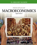
When the profitability of the firm decreases due to the increased nominal wage rate of the labor, the supply will decline in the economy, which will cause the short run aggregate supply curve to shift upward and this can be illustrated on the graph as follows:
Concept introduction:
Aggregate demand curve: It is the curve that shows the relationship between the price level in the economy and the quantity of real GDP demanded by the economic agents such as the households, firms, and the government.
Aggregate supply curve: In the short run, it is a curve that shows the relationship between the price level in the economy and the supply in the economy by the firms. In the long run, it shows the relationship between the price level and the level of quantity supplied by the firms.
Equilibrium: The equilibrium in the economy is the point where the economy's aggregate demand curve and the aggregate supply curve intersect with each other. There will be no excess demand or excess supply in the economy at the equilibrium.
Sub part (e):
Impact of different views on inflation on the economy's equilibrium.
Sub part (e):
Explanation of Solution
When the aggregate demand is held constant without any change and the aggregate supply shifts to AS2 as given above, it will lead to lower output in the economy along with higher price level in the economy. This is because when the SRAS curve shifts upward, the new equilibrium will be derived at point B, which is lying above and leftward to the initial equilibrium point A.
Concept introduction:
Aggregate demand curve: It is the curve that shows the relationship between the price level in the economy and the quantity of real GDP demanded by the economic agents such as the households, firms, and the government.
Aggregate supply curve: In the short run, it is a curve that shows the relationship between the price level in the economy and the supply in the economy by the firms. In the long run, it shows the relationship between the price level and the level of quantity supplied by the firms.
Equilibrium: The equilibrium in the economy is the point where the economy's aggregate demand curve and the aggregate supply curve intersect with each other. There will be no excess demand or excess supply in the economy at the equilibrium.
Sub part (f):
Impact of different views on inflation on the economy's equilibrium.
Sub part (f):
Explanation of Solution
The situation explained above that the total output of the economy falls, whereas the price level in the economy increases leading to the situation of stagflation and this means that the appointment choice of the new chairman was not a wise choice.
Concept introduction:
Aggregate demand curve: It is the curve that shows the relationship between the price level in the economy and the quantity of real GDP demanded by the economic agents such as the households, firms, and the government.
Aggregate supply curve: In the short run, it is a curve that shows the relationship between the price level in the economy and the supply in the economy by the firms. In the long run, it shows the relationship between the price level and the level of quantity supplied by the firms.
Equilibrium: The equilibrium in the economy is the point where the economy's aggregate demand curve and the aggregate supply curve intersect with each other. There will be no excess demand or excess supply in the economy at the equilibrium.
Want to see more full solutions like this?
Chapter 20 Solutions
EBK PRINCIPLES OF MACROECONOMICS

- I need help in seeing how these are the answers. If you could please write down your steps so I can see how it's done please.arrow_forwardSuppose that a random sample of 216 twenty-year-old men is selected from a population and that their heights and weights are recorded. A regression of weight on height yields Weight = (-107.3628) + 4.2552 x Height, R2 = 0.875, SER = 11.0160 (2.3220) (0.3348) where Weight is measured in pounds and Height is measured in inches. A man has a late growth spurt and grows 1.6200 inches over the course of a year. Construct a confidence interval of 90% for the person's weight gain. The 90% confidence interval for the person's weight gain is ( ☐ ☐) (in pounds). (Round your responses to two decimal places.)arrow_forwardSuppose that (Y, X) satisfy the assumptions specified here. A random sample of n = 498 is drawn and yields Ŷ= 6.47 + 5.66X, R2 = 0.83, SER = 5.3 (3.7) (3.4) Where the numbers in parentheses are the standard errors of the estimated coefficients B₁ = 6.47 and B₁ = 5.66 respectively. Suppose you wanted to test that B₁ is zero at the 5% level. That is, Ho: B₁ = 0 vs. H₁: B₁ #0 Report the t-statistic and p-value for this test. Definition The t-statistic is (Round your response to two decimal places) ☑ The Least Squares Assumptions Y=Bo+B₁X+u, i = 1,..., n, where 1. The error term u; has conditional mean zero given X;: E (u;|X;) = 0; 2. (Y;, X¡), i = 1,..., n, are independent and identically distributed (i.i.d.) draws from i their joint distribution; and 3. Large outliers are unlikely: X; and Y, have nonzero finite fourth moments.arrow_forward
- Asap pleasearrow_forwardTasks Exercise 1 Assess the following functions: 1. f(x)= x2+6x+2 2.f '(x)=10x-2x2+5 a. Find the stationary points. (5 marks) b. Determine whether the stationary point is a maximum or minimum. (5 marks) c. Draw the corresponding curves (5 marks)arrow_forwardProblem 2: The sales data over the last 10 years for the Acme Hardware Store are as follows: 2003 $230,000 2008 $526,000 2004 276,000 2009 605,000 2005 328,000 2010 690,000 2006 388,000 2011 779,000 2007 453,000 2012 873,000 1. Calculate the compound growth rate for the period of 2003 to 2012. 2. Based on your answer to part a, forecast sales for both 2013 and 2014. 3. Now calculate the compound growth rate for the period of 2007 to 2012. 1. Based on your answer to part e, forecast sales for both 2013 and 2014. 5. What is the major reason for the differences in your answers to parts b and d? If you were to make your own projections, what would you forecast? (Drawing a graph is very helpful.)arrow_forward
- Exercise 4A firm has the following average cost: AC = 200 + 2Q – 36 Q Find the stationary point and determine if it is a maximum or a minimum.b. Find the marginal cost function.arrow_forwardExercise 4A firm has the following average cost: AC = 200 + 2Q – 36 Q Find the stationary point and determine if it is a maximum or a minimum.b. Find the marginal cost function.arrow_forwardExercise 2A firm has the following short-run production function: Q = 30L2 -0.5L3a. Make a table with two columns: Production and Labour b. Add a third column to the table with the marginal product of labour c. Graph the values that you estimated for the production function and the marginal product oflabour Exercise 3A Firm has the following production function: Q= 20L-0.4L2a. Using differential calculus find the unit of labour that maximizes the production. b. Estimate function of Marginal product of labor c. Obtain the Average product of labor. d. Find the point at which the Marginal Product of Labour is equal to the Average Product of Labour.arrow_forward
- Problem 3 You have the following data for the last 12 months' sales for the PRQ Corporation (in thousands of dollars): January 500 July 610 February 520 August 620 March 520 September 580 April 510 October 550 May 530 November 510 June 580 December 480 1. Calculate a 3-month centered moving average. 2. Use this moving average to forecast sales for January of next year. 3. If you were asked to forecast January and February sales for next year, would you be confident of your forecast using the preceding moving averages? Why or why not? expect? Explain.arrow_forwardProblem 5 The MNO Corporation is preparing for its stockholder meeting on May 15, 2013. It sent out proxies to its stockholders on March 15 and asked stockholders who plan to attend the meeting to respond. To plan for a sufficient number of information packages to be distributed at the meeting, as well as for refreshments to be served, the company has asked you to forecast the number of attending stockholders. By April 15, 378 stockholders have expressed their intention to attend. You have available the following data for the last 6 years for total attendance at the stockholder meeting and the number of positive responses as of April 15: Year Positive Responses Attendance 2007 322 520 2008 301 550 2009 398 570 2010 421 600 2011 357 570 2012 452 650 1. What is your attendance forecast for the 2013 stockholder meeting? 2. Are there any other factors that could affect attendance, and thus make your forecast inac- curate?arrow_forwardProblem 4 Office Enterprises (OE) produces a line of metal office file cabinets. The company's economist, having investigated a large number of past data, has established the following equation of demand for these cabinets: Q=10,000+6013-100P+50C Q=Annual number of cabinets sold B = Index of nonresidential construction P = Average price per cabinet charged by OE C=Average price per cabinet charged by OE's closest competitor It is expected that next year's nonresidential construction index will stand at 160, OE's average price will be $40, and the competitor's average price will be $35. 1. Forecast next year's sales. 2. What will be the effect if the competitor lowers its price to 832? If it raises its price to $36? 3. What will happen if OE reacts to the decrease mentioned in part b by lowering its price to $37? 4. If the index forecast was wrong, and it turns out to be only 140 next year, what will be the effect on OE's sales? If not, what does it measure?arrow_forward
 Macroeconomics: Private and Public Choice (MindTa...EconomicsISBN:9781305506756Author:James D. Gwartney, Richard L. Stroup, Russell S. Sobel, David A. MacphersonPublisher:Cengage Learning
 Economics: Private and Public Choice (MindTap Cou...EconomicsISBN:9781305506725Author:James D. Gwartney, Richard L. Stroup, Russell S. Sobel, David A. MacphersonPublisher:Cengage Learning
 Exploring EconomicsEconomicsISBN:9781544336329Author:Robert L. SextonPublisher:SAGE Publications, Inc
 Economics (MindTap Course List)EconomicsISBN:9781337617383Author:Roger A. ArnoldPublisher:Cengage Learning