Subpart (a):
Long run equilibrium in AD-AS model.
Subpart (a):
Explanation of Solution
The supply depends upon the
The
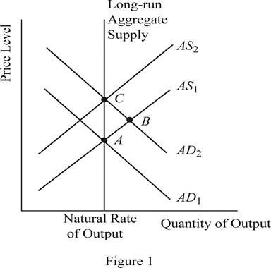
The equilibrium is a condition where the aggregate demand curve of the economy intersects with the aggregate supply curve of the economy. Then there will be an equilibrium point derived where the economy will be in its equilibrium without any excess demand or supply. The quantity on the X axis will represent the
Concept introduction:
Aggregate demand curve: It is the curve which shows the relationship between the price level in the economy and the quantity of real GDP demanded by the economic agents such as the households, firms as well as the government.
Equilibrium: The equilibrium in the economy is the point where the economy's aggregate demand curve and the aggregate supply curve intersects with each other. There will be no excess demand or
Subpart (b):
Long run equilibrium in AD-AS model.
Subpart (b):
Explanation of Solution
When the money supply of the economy increases with the intervention of the Central Bank of the economy, the money with the public will increase. When the money with the public increases, they will feel wealthier and as a result they will demand more consumer goods and services. As a result, the aggregate demand of the economy increases and it will shift the AD curve towards the right. This can be identified as the change to the equilibrium point B as shown in Figure 1. Thus, in short, the increase in the money supply leads to the increase in the output and price level of the economy.
Concept introduction:
Aggregate demand curve: It is the curve which shows the relationship between the price level in the economy and the quantity of real GDP demanded by the economic agents such as the households, firms as well as the government.
Aggregate supply curve: In the short run, it is a curve which shows the relationship between the price level in the economy and the supply in the economy by the firms. In the long run, it shows the relationship between the price level and the level of quantity supplied by the firms.
Equilibrium: The equilibrium in the economy is the point where the economy's aggregate demand curve and the aggregate supply curve intersects with each other. There will be no excess demand or excess supply in the economy at the equilibrium.
Subpart (c):
Long run equilibrium in AD-AS model.
Subpart (c):
Explanation of Solution
When the AD curve shifts towards the right and increases the output and the price level in the short run, over time, the nominal wages, prices as well as the perceptions and expectations of the economy would adjust to the new equilibrium level. As a result of this gradual adjustment, the cost of production will increase and the result will be a leftward shift in the aggregate supply curve of the economy. Then the economy will return to its natural level of output at a higher price level of the economy. This can be identified as the movement from point B to point C in the graph shown above.
Concept introduction:
Aggregate demand curve: It is the curve which shows the relationship between the price level in the economy and the quantity of real GDP demanded by the economic agents such as the households, firms as well as the government.
Aggregate supply curve: In the short run, it is a curve which shows the relationship between the price level in the economy and the supply in the economy by the firms. In the long run, it shows the relationship between the price level and the level of quantity supplied by the firms.
Equilibrium: The equilibrium in the economy is the point where the economy's aggregate demand curve and the aggregate supply curve intersects with each other. There will be no excess demand or excess supply in the economy at the equilibrium.
Subpart (d):
Long run equilibrium in AD-AS model.
Subpart (d):
Explanation of Solution
The sticky wages theory suggests that when there is inflation in the economy, the wage rate will adjust very slowly to the inflation. More or less the wage rates will be sticky and the main reason will be the long term contracts between the employer and the employees. Thus, in the short run equilibriums such as point A and point B, the wages of the economy would be more or less equal to each other. Whereas the point C represents the long run equilibrium and thus, the wages at the point C will be higher than that in point A and B.
Concept introduction:
Aggregate demand curve: It is the curve which shows the relationship between the price level in the economy and the quantity of real GDP demanded by the economic agents such as the households, firms as well as the government.
Aggregate supply curve: In the short run, it is a curve which shows the relationship between the price level in the economy and the supply in the economy by the firms. In the long run, it shows the relationship between the price level and the level of quantity supplied by the firms.
Equilibrium: The equilibrium in the economy is the point where the economy's aggregate demand curve and the aggregate supply curve intersects with each other. There will be no excess demand or excess supply in the economy at the equilibrium.
Subpart (e):
Long run equilibrium in AD-AS model.
Subpart (e):
Explanation of Solution
The sticky wages theory suggests that when there is inflation in the economy, the wage rate will adjust very slowly to the inflation. More or less, the wage rates will be sticky and the main reason will be the long term contracts between the employer and the employees. So, the nominal wages at equilibrium point A and B will be same. But the increase in the general price level in the economy would reduce the real wages of the workers because, the real wage is the nominal wage divided by the price level. When the denominator increases, it will reduce the value of the real wages in the economy.
Concept introduction:
Aggregate demand curve: It is the curve which shows the relationship between the price level in the economy and the quantity of real GDP demanded by the economic agents such as the households, firms as well as the government.
Aggregate supply curve: In the short run, it is a curve which shows the relationship between the price level in the economy and the supply in the economy by the firms. In the long run, it shows the relationship between the price level and the level of quantity supplied by the firms.
Equilibrium: The equilibrium in the economy is the point where the economy's aggregate demand curve and the aggregate supply curve intersects with each other. There will be no excess demand or excess supply in the economy at the equilibrium.
Sub part (f):
Long run equilibrium in AD-AS model.
Sub part (f):
Explanation of Solution
When the increase in the money supply happens in the economy, it will lead to the increase in the nominal wages as well as the price level in the economy in the long run. As a result of the increase in the nominal wage rate along with the price level in the economy, the real wage rate of the economy would remain unchanged. Thus, the neutrality of money applies in the long run equilibrium.
Concept introduction:
Aggregate demand curve: It is the curve which shows the relationship between the price level in the economy and the quantity of real GDP demanded by the economic agents such as the households, firms as well as the government.
Aggregate supply curve: In the short run, it is a curve which shows the relationship between the price level in the economy and the supply in the economy by the firms. In the long run, it shows the relationship between the price level and the level of quantity supplied by the firms.
Equilibrium: The equilibrium in the economy is the point where the economy's aggregate demand curve and the aggregate supply curve intersects with each other. There will be no excess demand or excess supply in the economy at the equilibrium.
Want to see more full solutions like this?
Chapter 20 Solutions
PRIN.OF MACROECON.(LL)-W/ACCESS>CUSTOM<

- Problem 3 You are given the following demand for European luxury automobiles: Q=1,000 P-0.5.2/1.6 where P-Price of European luxury cars PA = Price of American luxury cars P, Price of Japanese luxury cars I= Annual income of car buyers Assume that each of the coefficients is statistically significant (i.e., that they passed the t-test). On the basis of the information given, answer the following questions 1. Comment on the degree of substitutability between European and American luxury cars and between European and Japanese luxury cars. Explain some possible reasons for the results in the equation. 2. Comment on the coefficient for the income variable. Is this result what you would expect? Explain. 3. Comment on the coefficient of the European car price variable. Is that what you would expect? Explain.arrow_forwardProblem 2: A manufacturer of computer workstations gathered average monthly sales figures from its 56 branch offices and dealerships across the country and estimated the following demand for its product: Q=+15,000-2.80P+150A+0.3P+0.35Pm+0.2Pc (5,234) (1.29) (175) (0.12) (0.17) (0.13) R²=0.68 SER 786 F=21.25 The variables and their assumed values are P = Price of basic model = 7,000 Q==Quantity A = Advertising expenditures (in thousands) = 52 P = Average price of a personal computer = 4,000 P. Average price of a minicomputer = 15,000 Pe Average price of a leading competitor's workstation = 8,000 1. Compute the elasticities for each variable. On this basis, discuss the relative impact that each variable has on the demand. What implications do these results have for the firm's marketing and pricing policies? 2. Conduct a t-test for the statistical significance of each variable. In each case, state whether a one-tail or two-tail test is required. What difference, if any, does it make to…arrow_forwardYou are the manager of a large automobile dealership who wants to learn more about the effective- ness of various discounts offered to customers over the past 14 months. Following are the average negotiated prices for each month and the quantities sold of a basic model (adjusted for various options) over this period of time. 1. Graph this information on a scatter plot. Estimate the demand equation. What do the regression results indicate about the desirability of discounting the price? Explain. Month Price Quantity Jan. 12,500 15 Feb. 12,200 17 Mar. 11,900 16 Apr. 12,000 18 May 11,800 20 June 12,500 18 July 11,700 22 Aug. 12,100 15 Sept. 11,400 22 Oct. 11,400 25 Nov. 11,200 24 Dec. 11,000 30 Jan. 10,800 25 Feb. 10,000 28 2. What other factors besides price might be included in this equation? Do you foresee any difficulty in obtaining these additional data or incorporating them in the regression analysis?arrow_forward
- simple steps on how it should look like on excelarrow_forwardConsider options on a stock that does not pay dividends.The stock price is $100 per share, and the risk-free interest rate is 10%.Thestock moves randomly with u=1.25and d=1/u Use Excel to calculate the premium of a10-year call with a strike of $100.arrow_forwardCompute the Fourier sine and cosine transforms of f(x) = e.arrow_forward
- 17. Given that C=$700+0.8Y, I=$300, G=$600, what is Y if Y=C+I+G?arrow_forwardUse the Feynman technique throughout. Assume that you’re explaining the answer to someone who doesn’t know the topic at all. Write explanation in paragraphs and if you use currency use USD currency: 10. What is the mechanism or process that allows the expenditure multiplier to “work” in theKeynesian Cross Model? Explain and show both mathematically and graphically. What isthe underpinning assumption for the process to transpire?arrow_forwardUse the Feynman technique throughout. Assume that you’reexplaining the answer to someone who doesn’t know the topic at all. Write it all in paragraphs: 2. Give an overview of the equation of exchange (EoE) as used by Classical Theory. Now,carefully explain each variable in the EoE. What is meant by the “quantity theory of money”and how is it different from or the same as the equation of exchange?arrow_forward
 Essentials of Economics (MindTap Course List)EconomicsISBN:9781337091992Author:N. Gregory MankiwPublisher:Cengage Learning
 Principles of Economics (MindTap Course List)EconomicsISBN:9781305585126Author:N. Gregory MankiwPublisher:Cengage Learning
 Principles of Macroeconomics (MindTap Course List)EconomicsISBN:9781285165912Author:N. Gregory MankiwPublisher:Cengage Learning
 Brief Principles of Macroeconomics (MindTap Cours...EconomicsISBN:9781337091985Author:N. Gregory MankiwPublisher:Cengage Learning
 Principles of Economics, 7th Edition (MindTap Cou...EconomicsISBN:9781285165875Author:N. Gregory MankiwPublisher:Cengage Learning
 Principles of Macroeconomics (MindTap Course List)EconomicsISBN:9781305971509Author:N. Gregory MankiwPublisher:Cengage Learning