Subpart (a):
Long run equilibrium in AD-AS model.
Subpart (a):
Explanation of Solution
The supply depends upon the
The
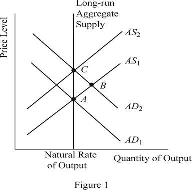
The equilibrium is a condition where the aggregate demand curve of the economy intersects with the aggregate supply curve of the economy. Then there will be an equilibrium point derived where the economy will be in its equilibrium without any excess demand or supply. The quantity on the X axis will represent the
Concept introduction:
Aggregate demand curve: It is the curve which shows the relationship between the price level in the economy and the quantity of real GDP demanded by the economic agents such as the households, firms as well as the government.
Equilibrium: The equilibrium in the economy is the point where the economy's aggregate demand curve and the aggregate supply curve intersects with each other. There will be no excess demand or
Subpart (b):
Long run equilibrium in AD-AS model.
Subpart (b):
Explanation of Solution
When the money supply of the economy increases with the intervention of the Central Bank of the economy, the money with the public will increase. When the money with the public increases, they will feel wealthier and as a result they will demand more consumer goods and services. As a result, the aggregate demand of the economy increases and it will shift the AD curve towards the right. This can be identified as the change to the equilibrium point B as shown in Figure 1. Thus, in short, the increase in the money supply leads to the increase in the output and price level of the economy.
Concept introduction:
Aggregate demand curve: It is the curve which shows the relationship between the price level in the economy and the quantity of real GDP demanded by the economic agents such as the households, firms as well as the government.
Aggregate supply curve: In the short run, it is a curve which shows the relationship between the price level in the economy and the supply in the economy by the firms. In the long run, it shows the relationship between the price level and the level of quantity supplied by the firms.
Equilibrium: The equilibrium in the economy is the point where the economy's aggregate demand curve and the aggregate supply curve intersects with each other. There will be no excess demand or excess supply in the economy at the equilibrium.
Subpart (c):
Long run equilibrium in AD-AS model.
Subpart (c):
Explanation of Solution
When the AD curve shifts towards the right and increases the output and the price level in the short run, over time, the nominal wages, prices as well as the perceptions and expectations of the economy would adjust to the new equilibrium level. As a result of this gradual adjustment, the cost of production will increase and the result will be a leftward shift in the aggregate supply curve of the economy. Then the economy will return to its natural level of output at a higher price level of the economy. This can be identified as the movement from point B to point C in the graph shown above.
Concept introduction:
Aggregate demand curve: It is the curve which shows the relationship between the price level in the economy and the quantity of real GDP demanded by the economic agents such as the households, firms as well as the government.
Aggregate supply curve: In the short run, it is a curve which shows the relationship between the price level in the economy and the supply in the economy by the firms. In the long run, it shows the relationship between the price level and the level of quantity supplied by the firms.
Equilibrium: The equilibrium in the economy is the point where the economy's aggregate demand curve and the aggregate supply curve intersects with each other. There will be no excess demand or excess supply in the economy at the equilibrium.
Subpart (d):
Long run equilibrium in AD-AS model.
Subpart (d):
Explanation of Solution
The sticky wages theory suggests that when there is inflation in the economy, the wage rate will adjust very slowly to the inflation. More or less the wage rates will be sticky and the main reason will be the long term contracts between the employer and the employees. Thus, in the short run equilibriums such as point A and point B, the wages of the economy would be more or less equal to each other. Whereas the point C represents the long run equilibrium and thus, the wages at the point C will be higher than that in point A and B.
Concept introduction:
Aggregate demand curve: It is the curve which shows the relationship between the price level in the economy and the quantity of real GDP demanded by the economic agents such as the households, firms as well as the government.
Aggregate supply curve: In the short run, it is a curve which shows the relationship between the price level in the economy and the supply in the economy by the firms. In the long run, it shows the relationship between the price level and the level of quantity supplied by the firms.
Equilibrium: The equilibrium in the economy is the point where the economy's aggregate demand curve and the aggregate supply curve intersects with each other. There will be no excess demand or excess supply in the economy at the equilibrium.
Subpart (e):
Long run equilibrium in AD-AS model.
Subpart (e):
Explanation of Solution
The sticky wages theory suggests that when there is inflation in the economy, the wage rate will adjust very slowly to the inflation. More or less, the wage rates will be sticky and the main reason will be the long term contracts between the employer and the employees. So, the nominal wages at equilibrium point A and B will be same. But the increase in the general price level in the economy would reduce the real wages of the workers because, the real wage is the nominal wage divided by the price level. When the denominator increases, it will reduce the value of the real wages in the economy.
Concept introduction:
Aggregate demand curve: It is the curve which shows the relationship between the price level in the economy and the quantity of real GDP demanded by the economic agents such as the households, firms as well as the government.
Aggregate supply curve: In the short run, it is a curve which shows the relationship between the price level in the economy and the supply in the economy by the firms. In the long run, it shows the relationship between the price level and the level of quantity supplied by the firms.
Equilibrium: The equilibrium in the economy is the point where the economy's aggregate demand curve and the aggregate supply curve intersects with each other. There will be no excess demand or excess supply in the economy at the equilibrium.
Sub part (f):
Long run equilibrium in AD-AS model.
Sub part (f):
Explanation of Solution
When the increase in the money supply happens in the economy, it will lead to the increase in the nominal wages as well as the price level in the economy in the long run. As a result of the increase in the nominal wage rate along with the price level in the economy, the real wage rate of the economy would remain unchanged. Thus, the neutrality of money applies in the long run equilibrium.
Concept introduction:
Aggregate demand curve: It is the curve which shows the relationship between the price level in the economy and the quantity of real GDP demanded by the economic agents such as the households, firms as well as the government.
Aggregate supply curve: In the short run, it is a curve which shows the relationship between the price level in the economy and the supply in the economy by the firms. In the long run, it shows the relationship between the price level and the level of quantity supplied by the firms.
Equilibrium: The equilibrium in the economy is the point where the economy's aggregate demand curve and the aggregate supply curve intersects with each other. There will be no excess demand or excess supply in the economy at the equilibrium.
Want to see more full solutions like this?
Chapter 20 Solutions
Bundle: Principles of Macroeconomics, Loose-leaf Version, 8th + LMS Integrated Aplia, 1 term Printed Access Card

- Name: Problem 1: Managerial Economics, Assignment 5 April 20, 2025 If the sales of your company have grown from $500,000 five years ago to $1,050,150 this year, what is the compound growth rate? If you expect your sales to grow at a rate of 10 percent for the next five years, what should they be five years from now?arrow_forward1. In this question, assume all dollar units are real dollars in billions. For example, $100 means $100 billion. Argentina thinks it can find $105 of domestic investment projects with a marginal product of capital (MPK) equal to 10% (each $1 invested in year 0 pays off $0.10 in every later year). Assume a world real interest rate r*is 5%, and initial external wealth W (W in year -1) is 0. a. You find that the formula on the lecture slide: > r*, which means that a country will ΔΟ AK take on investment projects as long as the marginal product of capital (MPK) is at least as high as the real interest rate. Using this formula, answer if Argentina should conduct the project. b. If the projects are not done, GDP = Q = C = $200 in all years. Compute the present value of Q and C. c. If Argentina conducts the projects (investing $105), what is the present value of Q and C? d. If Argentina conducts the projects, what is the present value of C? Is Argentina better off with the investment?arrow_forward2. Consider a world of two countries: Highland (H) and Lowland (L). Each country has an average output of 9 and desires to smooth consumption. All income takes the form of capital income and is fully consumed each period. Initially, there are two states of the world: Pandemic (P) and Flood (F) each occurring with 50% probability. Pandemic affects Highland and lowers the output there to 8, leaving Lowland unaffected with an output of 10. Flood affects Lowland and lowers the output there to 8, leaving Highland unaffected with an output of 10. a. Assume that households in each country own the entire capital stock of their own land. Fill in the numbers on the following table. Pandemic Highland's income Lowland's income Flood Variation about the mean b. Assume that each country owns 50% of the other country's capital. Fill in the numbers on the following table. Pandemic Flood Variation about the mean Highland's income Lowland's income c. Compare your answer to (a) and (b). Does…arrow_forward
- 3. This question explores IS and FX equilibria in a numerical example. a. The consumption function is C = 1.5 + 0.8(Y - T). What is the marginal propensity to consume (MPC)? What is the marginal propensity to save (MPS)? b. The trade balance is TB = 5 [1-()] - (0.2(Y-8). What is the marginal propensity to consume foreign goods (MPCF)? What is the marginal propensity to consume home goods(MPCH)? c. The investment function is I = 3 - 10i. What is investment when the interest rate is equal to 0.10=10%. d. Assume government spending is G. Add up the four components of demand and write down the expression for D. Make sure that you simplify the equation. e. Derive the equation for the good market equilibrium using Y = D.arrow_forward1. A firm has the following demand function: P = 60 – 0.5Q and its total cost is defined by TC= 13+ Qa. Find the maximum revenue b. Find the production to optimize the profit. c. Verify if the marginal revenue and marginal cost are the same at the profit-maximizing productionlevel. Exercise 6From the point of view of the firm, what decision criteria have been found relevant in the analysis ofproduction and profit? Provide two refernces with your answer.arrow_forward5. Some people find options expensive and use more complex structures to reduce the cost. For example, consider buying a call with a strike of $55 and selling a call with a strike of $60. a. What is the cost of establishing this combined position? b. What is the payoff of the combined position if the market price goes to $60? c. What is the payoff of the combined position if the market price goes to $100?arrow_forward
- 3. An investor has $1,000 to invest. They believe the price of the underlier will increase to $60 within one year. a. How many shares of stock could they buy with the $1,000 at the current price of $50, and how much would they make if the share price increased to $60? b. How many calls with a strike of $55 could they buy for the same $1,000, and how much would they make if the share price increased to $60? c. How much would they make (or lose) from the stock and from the calls if the share price declined to $40? 4. What is the premium on a call with a strike of $0.01? Why is the premium so close to the $50 share price?arrow_forward1. We want to examine the comparative statics of the Black Scholes model. Complete the following table using the Excel model from class or another of your choice. Provide the call premium and the put premium for each scenario. Underlier Risk-free Scenario price rate Volatility Time to expiration Strike Call premium Put premium Baseline $50 5% 25% 1 year $55 Higher strike $50 5% 25% 1 year $60 Higher volatility $50 5% 40% 1 year $55 Higher risk free $50 8% 25% 1 year $55 More time $50 5% 25% 2 years $55 2. Look at the baseline scenario. a. What is the probability that the call is exercised in the baseline scenario? b. What is the probability that the put is exercised? c. Explain why the probabilities sum to 1.arrow_forwardSome people say that since inflation can be reduced in the long run without an increase in unemployment, we should reduce inflation to zero. Others believe that a steady rate of inflation at, say, 3 percent, should be our goal. What are the pros and cons of these two arguments? What, in your opinion, are good long-run goals for reducing inflation and unemployment?arrow_forward
- Explain in words how investment multiplier and the interest sensitivity of aggregate demand affect the slope of the IS curve. Explain in words how and why the income and interest sensitivities of the demand for real balances affect the slope of the LM curve. According to the IS–LM model, what happens to the interest rate, income, consumption, and investment under the following circumstances?a. The central bank increases the money supply.b. The government increases government purchases.c. The government increases taxes.arrow_forwardSuppose that a person’s wealth is $50,000 and that her yearlyincome is $60,000. Also suppose that her money demand functionis given by Md = $Y10.35 - i2Derive the demand for bonds. Suppose the interest rate increases by 10 percentage points. What is the effect on her demand for bonds?b. What are the effects of an increase in income on her demand for money and her demand for bonds? Explain in wordsarrow_forwardImagine you are a world leader and you just viewed this presentation as part of the United Nations Sustainable Development Goal Meeting. Summarize your findings https://www.youtube.com/watch?v=v7WUpgPZzpIarrow_forward
 Essentials of Economics (MindTap Course List)EconomicsISBN:9781337091992Author:N. Gregory MankiwPublisher:Cengage Learning
 Principles of Economics (MindTap Course List)EconomicsISBN:9781305585126Author:N. Gregory MankiwPublisher:Cengage Learning
 Principles of Macroeconomics (MindTap Course List)EconomicsISBN:9781285165912Author:N. Gregory MankiwPublisher:Cengage Learning
 Brief Principles of Macroeconomics (MindTap Cours...EconomicsISBN:9781337091985Author:N. Gregory MankiwPublisher:Cengage Learning
 Principles of Economics, 7th Edition (MindTap Cou...EconomicsISBN:9781285165875Author:N. Gregory MankiwPublisher:Cengage Learning
 Principles of Macroeconomics (MindTap Course List)EconomicsISBN:9781305971509Author:N. Gregory MankiwPublisher:Cengage Learning