Chapter 20, Problem 21E

(a)

To determine

To find: The expected value of the size of a household.

Answer to Problem 21E

Solution: The expected size of the household is approximately 3.

Explanation of Solution

Calculation:

The expected value of any discrete random variable X is computed by using the following formula:

$E\left(X\right)={\displaystyle \sum _{X}x\times p\left(X=x\right)}$

where $p\left(X=x\right)$ is the probability that the random variable assumes value $x$.

Using the above formula of expectation and the provided probability distribution of the size of a household, the expected value of the size of a household $\left(X\right)$ is computed as follows:

$\begin{array}{c}E\left(X\right)=\left[\begin{array}{c}\left(1\times 0.28\right)+\left(2\times 0.34\right)+\left(3\times 0.16\right)+\left(4\times 0.13\right)\\ +\left(5\times 0.06\right)+\left(6\times 0.02\right)+\left(7\times 0.01\right)\end{array}\right]\\ =\left(0.28+0.68+0.48+0.52+0.3+0.12+0.07\right)\\ =2.45\end{array}$

(b)

To determine

To find: The number of households of size 2.

Answer to Problem 21E

Solution: There are 340 households of size 2.

Explanation of Solution

Calculation:

The number of households of size 2 is computed as follows:

$\begin{array}{c}\left(\begin{array}{l}\text{Number of households}\\ \text{ of size 2}\end{array}\right)=\left(\begin{array}{l}\text{Total number of households in the sample}\\ \times \text{Proportion of people in the household of size 2}\end{array}\right)\\ =1000\times 0.34\\ =340\end{array}$

To find: The number of households of sizes 3 to 7.

Solution: There are 380 households of sizes 3 to 7.

Explanation:

Calculation:

From the provided probability distribution, the proportion for the households of sizes 3 to 7 is calculated as follows:

$\begin{array}{c}\left(\begin{array}{l}\text{Proportion for the households}\\ \text{ of sizes 3 to 7}\end{array}\right)=0.16+0.13+0.06+0.02+0.01\\ =0.38\end{array}$

Now, the number of households of sizes 3 to 7 is calculated as follows:

$\begin{array}{c}\left(\begin{array}{l}\text{Number of households}\\ \text{ of sizes 3 to 7}\end{array}\right)=\left(\begin{array}{l}\text{Total number of households in the sample}\\ \times \text{Proportion of people in the households of sizes 3 to 7}\end{array}\right)\\ =1000\times 0.38\\ =380\end{array}$

(c)

To determine

To find: The number of people represented in the sample of 1000 households.

Answer to Problem 21E

Solution: A total number of 2450 people are represented by the sample.

Explanation of Solution

Calculation:

The number of people represented in the sample is calculated from the provided probability distribution as follows:

$\begin{array}{c}\left(\begin{array}{l}\text{Number of people}\\ \text{represented by the sample}\end{array}\right)=\left[\begin{array}{l}\text{Size of each household}\\ \times \text{Proportion of people in the household}\end{array}\right]\times \text{Sample size}\\ =\left[\begin{array}{l}\left(1\times 0.28\right)+\left(2\times 0.34\right)+\left(3\times 0.16\right)+\left(4\times 0.13\right)\\ +\left(5\times 0.06\right)+\left(6\times 0.02\right)+\left(7\times 0.01\right)\end{array}\right]\times 1000\\ =2.45\times 1000\\ =2450\end{array}$

(d)

To determine

To find: The probability distribution for household size and the shape of the obtained distribution.

Answer to Problem 21E

Solution: The required probability distribution is shown below:

$\begin{array}{cccccccc}\text{Family size}& 1& 2& 3& 4& 5& 6& 7\\ \text{Probability}& 0.1143& 0.2776& 0.1959& 0.2122& 0.1224& 0.0489& 0.0286\end{array}$

The shape of the distribution is rightskewed.

Explanation of Solution

Calculation:

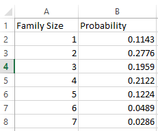
From the provided probability distribution, the family size is calculated as displayed in the table below:

$\begin{array}{ccc}\text{Family size}& \text{Proportion}& \text{Number of people }\\ 1& 0.28& 1\times 0.28\times 1000=280\\ 2& 0.34& 2\times 0.34\times 1000=680\\ 3& 0.16& 3\times 0.16\times 1000=480\\ 4& 0.13& 4\times 0.13\times 1000=520\\ 5& 0.06& 5\times 0.06\times 1000=300\\ 6& 0.02& 6\times 0.02\times 1000=120\\ 7& 0.01& 7\times 0.01\times 1000=70\end{array}$

The probability corresponding to each of the family size is computed as shown below:

$\begin{array}{ccc}\text{Family size}& \text{Number of people }& \text{Probability}\\ 1& 1\times 0.28\times 1000=280& \frac{280}{2450}=0.1143\\ 2& 2\times 0.34\times 1000=680& \frac{680}{2450}=0.2776\\ 3& 3\times 0.16\times 1000=480& \frac{480}{2450}=0.1959\\ 4& 4\times 0.13\times 1000=520& \frac{520}{2450}=0.2122\\ 5& 5\times 0.06\times 1000=300& \frac{300}{2450}=0.1224\\ 6& 6\times 0.02\times 1000=120& \frac{120}{2450}=0.0489\\ 7& 7\times 0.01\times 1000=70& \frac{70}{2450}=0.0286\end{array}$

Graph: Now to determine the shape of the above obtained probability distribution, enter the data in Excel as displayed below:

Next select the entered data and go to “Insert” and select the “2-D Column” as shown in the screenshot below:

The obtained bar chart is shown below:

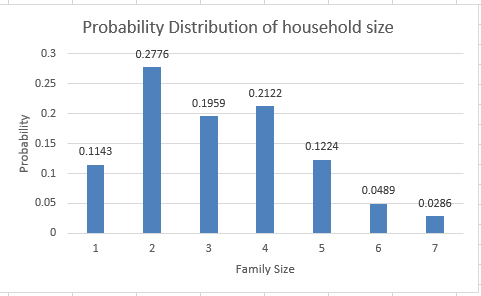
From the above graphical representation of the probability distribution, it is clear that the distribution is right skewed and as the family size increases the probability of the size of household decreases.

Interpretation: The probability distribution of the household size describes the probability associated with each of the household corresponding to the number of members living in it. The distribution is skewed toward right and it is concluded that the families of large size are less probable. Most of the households tend to have a size of 2.