
a.
To explain: Matched pairs design.
a.
Answer to Problem 20.33E
The newt’s ability to heal in one leg depends on the newt’s ability to heal in another leg. Moreover, the two hind limbs namely, control limb and experimental limb are matched by newt.
Explanation of Solution
Given info:
In the experiment, the two hind limbs of 12 newts were assigned at random to either experimental or control group.
Justification:
Matched pairs:
If the sample values from one population are associated or matched with the sample values from another population, then the two samples are said to be matched pairs or dependent samples.
Matched pair design occurs at two situations, which are listed below:
- Subjects are matched with pairs and each treatment is given to one subject in each pair
- Before and after observations on the same subjects.
In the given experiment, the newt’s ability to heal in one leg depends on the newt’s ability to heal in another leg. This indicates that the samples are not independent. Thus, the two hind limbs namely, control limb and experimental limb are matched by newt.
b.
To construct: The stemplot of the differences between limbs of the same newt and also to check whether there is a high outlier or not.
b.
Answer to Problem 20.33E
Output using the MINITAB software is given below:
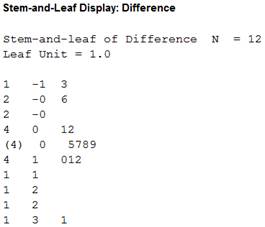
The stemplot plot clearly establishes the extreme outlier mentioned in the question.
Explanation of Solution
Calculation:
Software procedure:
Step-by-step procedure to construct the stemplot using the MINITAB software:
- Select Graph > Stem and leaf.
- In Graph variables, select Difference.
- Select OK
Interpretation:
There is sign of a major deviation from normality because the shape of the distribution is not a bell shape. That is, the stemplot suggests that the distribution of the data is skewed to the right with an extreme outlier (31). Thus, the stemplot plot clearly establishes the extreme outlier mentioned in the question.
c.
To find: The test statistic and P value with one test including all 12 newts and another omitting the outlier.
To check: Whether the outliers have a strong influence on conclusion or not.
c.
Answer to Problem 20.33E
There is sufficient evidence to support the claim for the
When omitting the outliers from the data set, there is weaker evidence to support the claim for the mean healing rate being significantly lower in the experimental limbs.
Yes, the outliers have a strong influence on the conclusion.
Explanation of Solution
Given info:
The mean healing rate is significantly lower in the experimental limbs with one test including all 12 newts and another omitting the outlier.
Calculation:
The null and alternative hypotheses are given below:
Null hypothesis:
Alternative hypothesis:
Test statistic and P-value for original data:
Software procedure:
Step-by-step procedure to obtain the test statistic and P-value for the original data using the MINITAB software:
- Choose Stat > Basic Statistics > 1-Sample t.
- In Samples in Column, enter the column of “Difference”.
- In Perform hypothesis test, enter the test mean as 0.
- Check Options, enter Confidence level as 95.0.
- Choose greater than in alternative.
- Click OK in all dialogue boxes.
Output using the MINITAB software is given below:
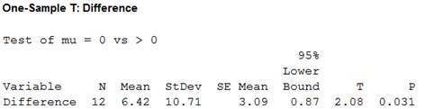
Thus, the test statistic is 2.08 and the P-value is 0.031.
Decision criteria for the P-value method:
If
If
Conclusion:
Here, the P-value for the hypotheses tests is 0.031, which is less than the level of significance. That is,
Test statistic and P-value when omitting the outlier:
Software procedure:
Step-by-step procedure to obtain the test statistic and P-value when omitting the outlier using the MINITAB software:
- Choose Stat > Basic Statistics > 1-Sample t.
- In Samples in Column, enter the column of “Difference”.
- In Perform hypothesis test, enter the test mean as 0.
- Check Options, enter Confidence level as 95.0.
- Choose greater than in alternative.
- Click OK in all dialogue boxes.
Output using the MINITAB software is given below:
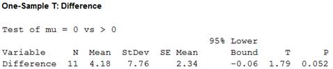
Thus, the test statistic is 1.79 and the P-value is 0.052.
Conclusion:
Here, the P-value for the hypotheses test is 0.052, which is greater than the level of significance. That is,
Comparison:
There is sufficient evidence to support the claim for the mean healing rate being significantly lower in the experimental limbs with all 12 differences. But, there is a weaker evidence to support the claim for the mean healing rate being significantly lower in the experimental limbs when omitting the outliers from the data set.
d.
To construct: The modified boxplot of the differences between the limbs of the same newt.
To find: The test statistic and P value with one test including all 12 newts and another omitting both the outliers.
To check: Whether the outliers have a strong influence on the conclusion or not.
To compare: The obtained test result with the result in part (c).
d.
Answer to Problem 20.33E
Output using the MINITAB software is given below:
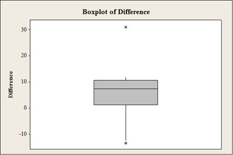
The graph suggests the distribution of the data skewed with two outliers.
Yes, the outliers have a strong influence on the conclusion.
When omitting the two outliers from the data set, there is stronger evidence to support the claim for the mean healing rate. It is significantly lower in the experimental limbs than the result in part (c).
Explanation of Solution
Calculation:
Software procedure:
Step-by-step procedure to construct the box plot for the original data using the MINITAB software:
- Choose Graph > Boxplot or Stat > EDA > Boxplot.
- Under Single Y, choose Simple. Click OK.
- In Graph variables, enter the data of Newts.
- Click OK.
Graph interpretation:
The boxplot suggests that the distribution of the data skewed with two extreme outliers (–13 and 31).
Test statistic and P-value after omitting the outliers:
Software procedure:
Step-by-step procedure to obtain the test statistic and P-value when omitting the outliers using the MINITAB software:
- Choose Stat > Basic Statistics > 1-Sample t.
- In Samples in Column, enter the column of “Difference”.
- In Perform hypothesis test, enter the test mean as 0.
- Check Options, enter Confidence level as 95.0.
- Choose greater than in alternative.
- Click OK in all dialogue boxes.
Output using the MINITAB software is given below:
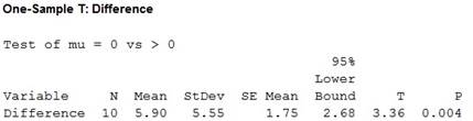
Thus, the test statistic is 3.36 and the P-value is 0.004.
Conclusion:
Here, the P-value for the hypotheses test is 0.004, which is less than the level of significance. That is,
Comparison:
There is strong evidence to support the claim for the mean healing rate being significantly lower in the experimental limbs after omitting the outliers from the data set when compared to the result in part (c).
Want to see more full solutions like this?
Chapter 20 Solutions
BASIC PRACTICE OF STATISTICS(REISSUE)>C

- ons 12. A sociologist hypothesizes that the crime rate is higher in areas with higher poverty rate and lower median income. She col- lects data on the crime rate (crimes per 100,000 residents), the poverty rate (in %), and the median income (in $1,000s) from 41 New England cities. A portion of the regression results is shown in the following table. Standard Coefficients error t stat p-value Intercept -301.62 549.71 -0.55 0.5864 Poverty 53.16 14.22 3.74 0.0006 Income 4.95 8.26 0.60 0.5526 a. b. Are the signs as expected on the slope coefficients? Predict the crime rate in an area with a poverty rate of 20% and a median income of $50,000. 3. Using data from 50 workarrow_forward2. The owner of several used-car dealerships believes that the selling price of a used car can best be predicted using the car's age. He uses data on the recent selling price (in $) and age of 20 used sedans to estimate Price = Po + B₁Age + ε. A portion of the regression results is shown in the accompanying table. Standard Coefficients Intercept 21187.94 Error 733.42 t Stat p-value 28.89 1.56E-16 Age -1208.25 128.95 -9.37 2.41E-08 a. What is the estimate for B₁? Interpret this value. b. What is the sample regression equation? C. Predict the selling price of a 5-year-old sedan.arrow_forwardian income of $50,000. erty rate of 13. Using data from 50 workers, a researcher estimates Wage = Bo+B,Education + B₂Experience + B3Age+e, where Wage is the hourly wage rate and Education, Experience, and Age are the years of higher education, the years of experience, and the age of the worker, respectively. A portion of the regression results is shown in the following table. ni ogolloo bash 1 Standard Coefficients error t stat p-value Intercept 7.87 4.09 1.93 0.0603 Education 1.44 0.34 4.24 0.0001 Experience 0.45 0.14 3.16 0.0028 Age -0.01 0.08 -0.14 0.8920 a. Interpret the estimated coefficients for Education and Experience. b. Predict the hourly wage rate for a 30-year-old worker with four years of higher education and three years of experience.arrow_forward
- 1. If a firm spends more on advertising, is it likely to increase sales? Data on annual sales (in $100,000s) and advertising expenditures (in $10,000s) were collected for 20 firms in order to estimate the model Sales = Po + B₁Advertising + ε. A portion of the regression results is shown in the accompanying table. Intercept Advertising Standard Coefficients Error t Stat p-value -7.42 1.46 -5.09 7.66E-05 0.42 0.05 8.70 7.26E-08 a. Interpret the estimated slope coefficient. b. What is the sample regression equation? C. Predict the sales for a firm that spends $500,000 annually on advertising.arrow_forwardCan you help me solve problem 38 with steps im stuck.arrow_forwardHow do the samples hold up to the efficiency test? What percentages of the samples pass or fail the test? What would be the likelihood of having the following specific number of efficiency test failures in the next 300 processors tested? 1 failures, 5 failures, 10 failures and 20 failures.arrow_forward
- The battery temperatures are a major concern for us. Can you analyze and describe the sample data? What are the average and median temperatures? How much variability is there in the temperatures? Is there anything that stands out? Our engineers’ assumption is that the temperature data is normally distributed. If that is the case, what would be the likelihood that the Safety Zone temperature will exceed 5.15 degrees? What is the probability that the Safety Zone temperature will be less than 4.65 degrees? What is the actual percentage of samples that exceed 5.25 degrees or are less than 4.75 degrees? Is the manufacturing process producing units with stable Safety Zone temperatures? Can you check if there are any apparent changes in the temperature pattern? Are there any outliers? A closer look at the Z-scores should help you in this regard.arrow_forwardNeed help pleasearrow_forwardPlease conduct a step by step of these statistical tests on separate sheets of Microsoft Excel. If the calculations in Microsoft Excel are incorrect, the null and alternative hypotheses, as well as the conclusions drawn from them, will be meaningless and will not receive any points. 4. One-Way ANOVA: Analyze the customer satisfaction scores across four different product categories to determine if there is a significant difference in means. (Hints: The null can be about maintaining status-quo or no difference among groups) H0 = H1=arrow_forward
- Please conduct a step by step of these statistical tests on separate sheets of Microsoft Excel. If the calculations in Microsoft Excel are incorrect, the null and alternative hypotheses, as well as the conclusions drawn from them, will be meaningless and will not receive any points 2. Two-Sample T-Test: Compare the average sales revenue of two different regions to determine if there is a significant difference. (Hints: The null can be about maintaining status-quo or no difference among groups; if alternative hypothesis is non-directional use the two-tailed p-value from excel file to make a decision about rejecting or not rejecting null) H0 = H1=arrow_forwardPlease conduct a step by step of these statistical tests on separate sheets of Microsoft Excel. If the calculations in Microsoft Excel are incorrect, the null and alternative hypotheses, as well as the conclusions drawn from them, will be meaningless and will not receive any points 3. Paired T-Test: A company implemented a training program to improve employee performance. To evaluate the effectiveness of the program, the company recorded the test scores of 25 employees before and after the training. Determine if the training program is effective in terms of scores of participants before and after the training. (Hints: The null can be about maintaining status-quo or no difference among groups; if alternative hypothesis is non-directional, use the two-tailed p-value from excel file to make a decision about rejecting or not rejecting the null) H0 = H1= Conclusion:arrow_forwardPlease conduct a step by step of these statistical tests on separate sheets of Microsoft Excel. If the calculations in Microsoft Excel are incorrect, the null and alternative hypotheses, as well as the conclusions drawn from them, will be meaningless and will not receive any points. The data for the following questions is provided in Microsoft Excel file on 4 separate sheets. Please conduct these statistical tests on separate sheets of Microsoft Excel. If the calculations in Microsoft Excel are incorrect, the null and alternative hypotheses, as well as the conclusions drawn from them, will be meaningless and will not receive any points. 1. One Sample T-Test: Determine whether the average satisfaction rating of customers for a product is significantly different from a hypothetical mean of 75. (Hints: The null can be about maintaining status-quo or no difference; If your alternative hypothesis is non-directional (e.g., μ≠75), you should use the two-tailed p-value from excel file to…arrow_forward
 MATLAB: An Introduction with ApplicationsStatisticsISBN:9781119256830Author:Amos GilatPublisher:John Wiley & Sons Inc
 Probability and Statistics for Engineering and th...StatisticsISBN:9781305251809Author:Jay L. DevorePublisher:Cengage Learning
 Statistics for The Behavioral Sciences (MindTap C...StatisticsISBN:9781305504912Author:Frederick J Gravetter, Larry B. WallnauPublisher:Cengage Learning
 Elementary Statistics: Picturing the World (7th E...StatisticsISBN:9780134683416Author:Ron Larson, Betsy FarberPublisher:PEARSON
 The Basic Practice of StatisticsStatisticsISBN:9781319042578Author:David S. Moore, William I. Notz, Michael A. FlignerPublisher:W. H. Freeman
 Introduction to the Practice of StatisticsStatisticsISBN:9781319013387Author:David S. Moore, George P. McCabe, Bruce A. CraigPublisher:W. H. Freeman