
a.
To explain: Matched pairs design.
a.
Answer to Problem 20.33E
The newt’s ability to heal in one leg depends on the newt’s ability to heal in another leg. Moreover, the two hind limbs namely, control limb and experimental limb are matched by newt.
Explanation of Solution
Given info:
In the experiment, the two hind limbs of 12 newts were assigned at random to either experimental or control group.
Justification:
Matched pairs:
If the sample values from one population are associated or matched with the sample values from another population, then the two samples are said to be matched pairs or dependent samples.
Matched pair design occurs at two situations, which are listed below:
- Subjects are matched with pairs and each treatment is given to one subject in each pair
- Before and after observations on the same subjects.
In the given experiment, the newt’s ability to heal in one leg depends on the newt’s ability to heal in another leg. This indicates that the samples are not independent. Thus, the two hind limbs namely, control limb and experimental limb are matched by newt.
b.
To construct: The stemplot of the differences between limbs of the same newt and also to check whether there is a high outlier or not.
b.
Answer to Problem 20.33E
Output using the MINITAB software is given below:
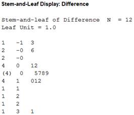
The stemplot plot clearly establishes the extreme outlier mentioned in the question.
Explanation of Solution
Calculation:
Software procedure:
Step-by-step procedure to construct the stemplot using the MINITAB software:
- Select Graph > Stem and leaf.
- In Graph variables, select Difference.
- Select OK
Interpretation:
There is sign of a major deviation from normality because the shape of the distribution is not a bell shape. That is, the stemplot suggests that the distribution of the data is skewed to the right with an extreme outlier (31). Thus, the stemplot plot clearly establishes the extreme outlier mentioned in the question.
c.
To find: The test statistic and P value with one test including all 12 newts and another omitting the outlier.
To check: Whether the outliers have a strong influence on conclusion or not.
c.
Answer to Problem 20.33E
There is sufficient evidence to support the claim for the
When omitting the outliers from the data set, there is weaker evidence to support the claim for the mean healing rate being significantly lower in the experimental limbs.
Yes, the outliers have a strong influence on the conclusion.
Explanation of Solution
Given info:
The mean healing rate is significantly lower in the experimental limbs with one test including all 12 newts and another omitting the outlier.
Calculation:
The null and alternative hypotheses are given below:
Null hypothesis:
Alternative hypothesis:
Test statistic and P-value for original data:
Software procedure:
Step-by-step procedure to obtain the test statistic and P-value for the original data using the MINITAB software:
- Choose Stat > Basic Statistics > 1-Sample t.
- In Samples in Column, enter the column of “Difference”.
- In Perform hypothesis test, enter the test mean as 0.
- Check Options, enter Confidence level as 95.0.
- Choose greater than in alternative.
- Click OK in all dialogue boxes.
Output using the MINITAB software is given below:
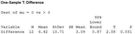
Thus, the test statistic is 2.08 and the P-value is 0.031.
Decision criteria for the P-value method:
If
If
Conclusion:
Here, the P-value for the hypotheses tests is 0.031, which is less than the level of significance. That is,
Test statistic and P-value when omitting the outlier:
Software procedure:
Step-by-step procedure to obtain the test statistic and P-value when omitting the outlier using the MINITAB software:
- Choose Stat > Basic Statistics > 1-Sample t.
- In Samples in Column, enter the column of “Difference”.
- In Perform hypothesis test, enter the test mean as 0.
- Check Options, enter Confidence level as 95.0.
- Choose greater than in alternative.
- Click OK in all dialogue boxes.
Output using the MINITAB software is given below:
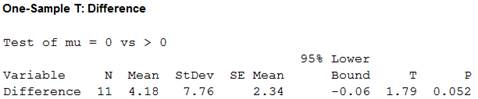
Thus, the test statistic is 1.79 and the P-value is 0.052.
Conclusion:
Here, the P-value for the hypotheses test is 0.052, which is greater than the level of significance. That is,
Comparison:
There is sufficient evidence to support the claim for the mean healing rate being significantly lower in the experimental limbs with all 12 differences. But, there is a weaker evidence to support the claim for the mean healing rate being significantly lower in the experimental limbs when omitting the outliers from the data set.
d.
To construct: The modified boxplot of the differences between the limbs of the same newt.
To find: The test statistic and P value with one test including all 12 newts and another omitting both the outliers.
To check: Whether the outliers have a strong influence on the conclusion or not.
To compare: The obtained test result with the result in part (c).
d.
Answer to Problem 20.33E
Output using the MINITAB software is given below:
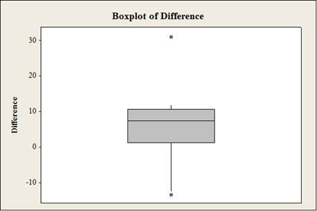
The graph suggests the distribution of the data skewed with two outliers.
Yes, the outliers have a strong influence on the conclusion.
When omitting the two outliers from the data set, there is stronger evidence to support the claim for the mean healing rate. It is significantly lower in the experimental limbs than the result in part (c).
Explanation of Solution
Calculation:
Software procedure:
Step-by-step procedure to construct the box plot for the original data using the MINITAB software:
- Choose Graph > Boxplot or Stat > EDA > Boxplot.
- Under Single Y, choose Simple. Click OK.
- In Graph variables, enter the data of Newts.
- Click OK.
Graph interpretation:
The boxplot suggests that the distribution of the data skewed with two extreme outliers (–13 and 31).
Test statistic and P-value after omitting the outliers:
Software procedure:
Step-by-step procedure to obtain the test statistic and P-value when omitting the outliers using the MINITAB software:
- Choose Stat > Basic Statistics > 1-Sample t.
- In Samples in Column, enter the column of “Difference”.
- In Perform hypothesis test, enter the test mean as 0.
- Check Options, enter Confidence level as 95.0.
- Choose greater than in alternative.
- Click OK in all dialogue boxes.
Output using the MINITAB software is given below:
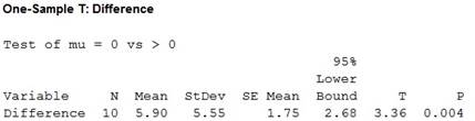
Thus, the test statistic is 3.36 and the P-value is 0.004.
Conclusion:
Here, the P-value for the hypotheses test is 0.004, which is less than the level of significance. That is,
Comparison:
There is strong evidence to support the claim for the mean healing rate being significantly lower in the experimental limbs after omitting the outliers from the data set when compared to the result in part (c).
Want to see more full solutions like this?
Chapter 20 Solutions
BASIC PRACTICE OF STATISTICS+LAUNCHPAD

- Review a classmate's Main Post. 1. State if you agree or disagree with the choices made for additional analysis that can be done beyond the frequency table. 2. Choose a measure of central tendency (mean, median, mode) that you would like to compute with the data beyond the frequency table. Complete either a or b below. a. Explain how that analysis can help you understand the data better. b. If you are currently unable to do that analysis, what do you think you could do to make it possible? If you do not think you can do anything, explain why it is not possible.arrow_forward0|0|0|0 - Consider the time series X₁ and Y₁ = (I – B)² (I – B³)Xt. What transformations were performed on Xt to obtain Yt? seasonal difference of order 2 simple difference of order 5 seasonal difference of order 1 seasonal difference of order 5 simple difference of order 2arrow_forwardCalculate the 90% confidence interval for the population mean difference using the data in the attached image. I need to see where I went wrong.arrow_forward
- Microsoft Excel snapshot for random sampling: Also note the formula used for the last column 02 x✓ fx =INDEX(5852:58551, RANK(C2, $C$2:$C$51)) A B 1 No. States 2 1 ALABAMA Rand No. 0.925957526 3 2 ALASKA 0.372999976 4 3 ARIZONA 0.941323044 5 4 ARKANSAS 0.071266381 Random Sample CALIFORNIA NORTH CAROLINA ARKANSAS WASHINGTON G7 Microsoft Excel snapshot for systematic sampling: xfx INDEX(SD52:50551, F7) A B E F G 1 No. States Rand No. Random Sample population 50 2 1 ALABAMA 0.5296685 NEW HAMPSHIRE sample 10 3 2 ALASKA 0.4493186 OKLAHOMA k 5 4 3 ARIZONA 0.707914 KANSAS 5 4 ARKANSAS 0.4831379 NORTH DAKOTA 6 5 CALIFORNIA 0.7277162 INDIANA Random Sample Sample Name 7 6 COLORADO 0.5865002 MISSISSIPPI 8 7:ONNECTICU 0.7640596 ILLINOIS 9 8 DELAWARE 0.5783029 MISSOURI 525 10 15 INDIANA MARYLAND COLORADOarrow_forwardSuppose the Internal Revenue Service reported that the mean tax refund for the year 2022 was $3401. Assume the standard deviation is $82.5 and that the amounts refunded follow a normal probability distribution. Solve the following three parts? (For the answer to question 14, 15, and 16, start with making a bell curve. Identify on the bell curve where is mean, X, and area(s) to be determined. 1.What percent of the refunds are more than $3,500? 2. What percent of the refunds are more than $3500 but less than $3579? 3. What percent of the refunds are more than $3325 but less than $3579?arrow_forwardA normal distribution has a mean of 50 and a standard deviation of 4. Solve the following three parts? 1. Compute the probability of a value between 44.0 and 55.0. (The question requires finding probability value between 44 and 55. Solve it in 3 steps. In the first step, use the above formula and x = 44, calculate probability value. In the second step repeat the first step with the only difference that x=55. In the third step, subtract the answer of the first part from the answer of the second part.) 2. Compute the probability of a value greater than 55.0. Use the same formula, x=55 and subtract the answer from 1. 3. Compute the probability of a value between 52.0 and 55.0. (The question requires finding probability value between 52 and 55. Solve it in 3 steps. In the first step, use the above formula and x = 52, calculate probability value. In the second step repeat the first step with the only difference that x=55. In the third step, subtract the answer of the first part from the…arrow_forward
- If a uniform distribution is defined over the interval from 6 to 10, then answer the followings: What is the mean of this uniform distribution? Show that the probability of any value between 6 and 10 is equal to 1.0 Find the probability of a value more than 7. Find the probability of a value between 7 and 9. The closing price of Schnur Sporting Goods Inc. common stock is uniformly distributed between $20 and $30 per share. What is the probability that the stock price will be: More than $27? Less than or equal to $24? The April rainfall in Flagstaff, Arizona, follows a uniform distribution between 0.5 and 3.00 inches. What is the mean amount of rainfall for the month? What is the probability of less than an inch of rain for the month? What is the probability of exactly 1.00 inch of rain? What is the probability of more than 1.50 inches of rain for the month? The best way to solve this problem is begin by a step by step creating a chart. Clearly mark the range, identifying the…arrow_forwardClient 1 Weight before diet (pounds) Weight after diet (pounds) 128 120 2 131 123 3 140 141 4 178 170 5 121 118 6 136 136 7 118 121 8 136 127arrow_forwardClient 1 Weight before diet (pounds) Weight after diet (pounds) 128 120 2 131 123 3 140 141 4 178 170 5 121 118 6 136 136 7 118 121 8 136 127 a) Determine the mean change in patient weight from before to after the diet (after – before). What is the 95% confidence interval of this mean difference?arrow_forward
- In order to find probability, you can use this formula in Microsoft Excel: The best way to understand and solve these problems is by first drawing a bell curve and marking key points such as x, the mean, and the areas of interest. Once marked on the bell curve, figure out what calculations are needed to find the area of interest. =NORM.DIST(x, Mean, Standard Dev., TRUE). When the question mentions “greater than” you may have to subtract your answer from 1. When the question mentions “between (two values)”, you need to do separate calculation for both values and then subtract their results to get the answer. 1. Compute the probability of a value between 44.0 and 55.0. (The question requires finding probability value between 44 and 55. Solve it in 3 steps. In the first step, use the above formula and x = 44, calculate probability value. In the second step repeat the first step with the only difference that x=55. In the third step, subtract the answer of the first part from the…arrow_forwardIf a uniform distribution is defined over the interval from 6 to 10, then answer the followings: What is the mean of this uniform distribution? Show that the probability of any value between 6 and 10 is equal to 1.0 Find the probability of a value more than 7. Find the probability of a value between 7 and 9. The closing price of Schnur Sporting Goods Inc. common stock is uniformly distributed between $20 and $30 per share. What is the probability that the stock price will be: More than $27? Less than or equal to $24? The April rainfall in Flagstaff, Arizona, follows a uniform distribution between 0.5 and 3.00 inches. What is the mean amount of rainfall for the month? What is the probability of less than an inch of rain for the month? What is the probability of exactly 1.00 inch of rain? What is the probability of more than 1.50 inches of rain for the month? The best way to solve this problem is begin by creating a chart. Clearly mark the range, identifying the lower and upper…arrow_forwardProblem 1: The mean hourly pay of an American Airlines flight attendant is normally distributed with a mean of 40 per hour and a standard deviation of 3.00 per hour. What is the probability that the hourly pay of a randomly selected flight attendant is: Between the mean and $45 per hour? More than $45 per hour? Less than $32 per hour? Problem 2: The mean of a normal probability distribution is 400 pounds. The standard deviation is 10 pounds. What is the area between 415 pounds and the mean of 400 pounds? What is the area between the mean and 395 pounds? What is the probability of randomly selecting a value less than 395 pounds? Problem 3: In New York State, the mean salary for high school teachers in 2022 was 81,410 with a standard deviation of 9,500. Only Alaska’s mean salary was higher. Assume New York’s state salaries follow a normal distribution. What percent of New York State high school teachers earn between 70,000 and 75,000? What percent of New York State high school…arrow_forward
 MATLAB: An Introduction with ApplicationsStatisticsISBN:9781119256830Author:Amos GilatPublisher:John Wiley & Sons Inc
 Probability and Statistics for Engineering and th...StatisticsISBN:9781305251809Author:Jay L. DevorePublisher:Cengage Learning
 Statistics for The Behavioral Sciences (MindTap C...StatisticsISBN:9781305504912Author:Frederick J Gravetter, Larry B. WallnauPublisher:Cengage Learning
 Elementary Statistics: Picturing the World (7th E...StatisticsISBN:9780134683416Author:Ron Larson, Betsy FarberPublisher:PEARSON
 The Basic Practice of StatisticsStatisticsISBN:9781319042578Author:David S. Moore, William I. Notz, Michael A. FlignerPublisher:W. H. Freeman
 Introduction to the Practice of StatisticsStatisticsISBN:9781319013387Author:David S. Moore, George P. McCabe, Bruce A. CraigPublisher:W. H. Freeman