Concept explainers
Videos
(a)
To graph: The
(a)
Explanation of Solution
Graph: To draw the scatterplot for the provided data set, the below steps are followed in Minitab software.
Step 1: Open the “MEIS” file in Minitab software.
Step 2: Go to Graph
Step 3: Choose the option “Simple” and click “OK”.
Step 4: Select “Sales” as Y variables and “Dwellpermit” as X variables.
Step 5: Click “OK” twice.
The scatterplot is obtained as:
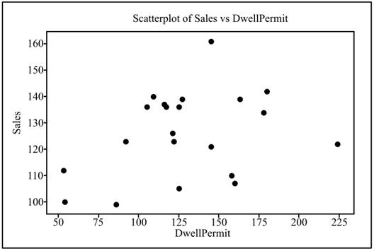
To explain: The relationship between the variables and the presence of the outliers.
Answer to Problem 144E
Solution: Though the relationship between the variables is very weak, but there is no outlier in the data set.
Explanation of Solution
(b)
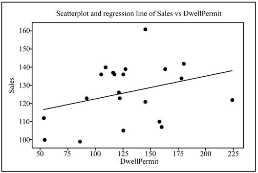
To find: The least-squares regression line for the data.
(b)
Answer to Problem 144E
Solution: The least-squares regression line is obtained as
Explanation of Solution
Calculation: To draw the regression line and obtain the sketch of the regression line, the below steps are followed in the Minitab software.
Step 1: Right click on the obtained graph in the part (a).
Step 2: Go to Add
Step 3: Click on “Linear” under the menu “Model Order” and tick the “Fit intercept”.
Step 4: Click on “OK” to obtain the regression line.
The obtained regression equation is
Graph: The below graph shows the regression line.

(c)
To explain: The slope of the obtained line.
(c)
Answer to Problem 144E
Solution: The slope can be interpreted as if there is an increase of 1unit of the variable, issued permit for dwelling then there is an increase of 0.1263 units in the value of the variable sales.
Explanation of Solution
(d)
To explain: The intercept of the line.
(d)
Answer to Problem 144E
Solution: The intercept can be interpreted as the value of the response variable when the value of the explanatory variable is zero. As the value of the response variable is 109.8 for the zero issued permits, it is appropriate to use the intercept for explaining the relationship between the variables.
Explanation of Solution
(e)
The sales for an index of 224 dwelling permits.
(e)
Answer to Problem 144E
Solution: The predicted value of the sales is 138.0912.
Explanation of Solution
The predicted value can be calculated as:
(f)
To find: The residual value for Canada.
(f)
Answer to Problem 144E
Solution: The obtained value of the residual is
Explanation of Solution
Calculation: The sale for the Canada is provided as 122. The residual value for the sales for Canada whose index of dwelling permits is 224 is calculated as:
(g)
The percentage of variability in sales is explained by dwelling permit.
(g)
Answer to Problem 144E
Solution: The explained percentage of variability in sales is 10.30%.
Explanation of Solution
Therefore, the proportion of variation that is explained by the explanatory variables of the model is 10.30%.
Want to see more full solutions like this?
Chapter 2 Solutions
EBK INTRODUCTION TO THE PRACTICE OF STA


- Should you be confident in applying your regression equation to estimate the heart rate of a python at 35°C? Why or why not?arrow_forwardGiven your fitted regression line, what would be the residual for snake #5 (10 C)?arrow_forwardCalculate the 95% confidence interval around your estimate of r using Fisher’s z-transformation. In your final answer, make sure to back-transform to the original units.arrow_forward
- BUSINESS DISCUSSarrow_forwardA researcher wishes to estimate, with 90% confidence, the population proportion of adults who support labeling legislation for genetically modified organisms (GMOs). Her estimate must be accurate within 4% of the true proportion. (a) No preliminary estimate is available. Find the minimum sample size needed. (b) Find the minimum sample size needed, using a prior study that found that 65% of the respondents said they support labeling legislation for GMOs. (c) Compare the results from parts (a) and (b). ... (a) What is the minimum sample size needed assuming that no prior information is available? n = (Round up to the nearest whole number as needed.)arrow_forwardThe table available below shows the costs per mile (in cents) for a sample of automobiles. At a = 0.05, can you conclude that at least one mean cost per mile is different from the others? Click on the icon to view the data table. Let Hss, HMS, HLS, Hsuv and Hмy represent the mean costs per mile for small sedans, medium sedans, large sedans, SUV 4WDs, and minivans respectively. What are the hypotheses for this test? OA. Ho: Not all the means are equal. Ha Hss HMS HLS HSUV HMV B. Ho Hss HMS HLS HSUV = μMV Ha: Hss *HMS *HLS*HSUV * HMV C. Ho Hss HMS HLS HSUV =μMV = = H: Not all the means are equal. D. Ho Hss HMS HLS HSUV HMV Ha Hss HMS HLS =HSUV = HMVarrow_forward
 MATLAB: An Introduction with ApplicationsStatisticsISBN:9781119256830Author:Amos GilatPublisher:John Wiley & Sons Inc
 Probability and Statistics for Engineering and th...StatisticsISBN:9781305251809Author:Jay L. DevorePublisher:Cengage Learning
 Statistics for The Behavioral Sciences (MindTap C...StatisticsISBN:9781305504912Author:Frederick J Gravetter, Larry B. WallnauPublisher:Cengage Learning
 Elementary Statistics: Picturing the World (7th E...StatisticsISBN:9780134683416Author:Ron Larson, Betsy FarberPublisher:PEARSON
 The Basic Practice of StatisticsStatisticsISBN:9781319042578Author:David S. Moore, William I. Notz, Michael A. FlignerPublisher:W. H. Freeman
 Introduction to the Practice of StatisticsStatisticsISBN:9781319013387Author:David S. Moore, George P. McCabe, Bruce A. CraigPublisher:W. H. Freeman