Chapter 19, Problem 6P

Construct amplitude and phase line spectra for Prob. 19.4.

To determine

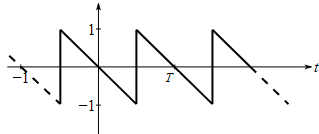
To graph: The amplitude and phase line spectra for the sawtooth wave as shown in the following figure,

Explanation of Solution

Given Information: The sawtooth wave given in the following figure,

Formula used:

Consider $f\left(t\right)$ is a periodic function with period $T$ defined in the interval $0\le x\le T$

then the Fourier series expansion of the function,

$f\left(t\right)=a_0+{\displaystyle \sum _{k=1}^{\infty }\left[a_k\cos \left(k{\omega }_{0}t\right)+b_k\sin \left(k{\omega }_{0}t\right)\right]}$ with ${\omega }_0=\frac{2\pi }{T}$.

And the coefficients are defined by,

$a_0=\frac{1}{T}{\displaystyle \underset{0}{\overset{T}{\int }}f\left(t\right)dt};a_k=\frac{2}{T}{\displaystyle \underset{0}{\overset{T}{\int }}f\left(t\right)\cos \left(k{\omega }_{0}t\right)dt};b_k=\frac{2}{T}{\displaystyle \underset{0}{\overset{T}{\int }}f\left(t\right)\sin \left(k{\omega }_{0}t\right)dt}$

Alternatively, the Fourier series can also be written as, $f\left(t\right)=a_0+{\displaystyle \sum _{k=1}^{\infty }\left[c_k\cos \left(k{\omega }_{0}t-{\varphi }_k\right)\right]}$

Here, the amplitude $c_k$ and phase ${\varphi }_k$ for each term is defined as,

$c_k^2=\sqrt{a_k^2+b_k^2},{\varphi }_k={\tan }^{-1}\left(\frac{b_k}{a_k}\right)$

Plot $c_k$ and ${\varphi }_k$ in the frequency domain to plot the amplitude and phase line spectra.

Graph:

Consider the sawtooth wave given in the following figure,

Therefore, the sawtooth wave is a periodic function $f\left(t\right)$ with period $T$ in the interval $0\le t\le T$ and from the graph,

$f\left(t\right)$ is a straight line joining the points $\left(0,0\right)$ and $\left(\frac{T}{2},-1\right)$ in $0\le t\le \frac{T}{2}$.

$f\left(t\right)$ is a straight line joining the points $\left(\frac{T}{2},1\right)$ and $\left(T,0\right)$ in $\frac{T}{2}\le t\le T$.

Therefore, the sawtooth wave,

$f\left(t\right)=\{\begin{array}{cc}-\frac{2}{T}t& 0\le t\le \frac{T}{2}\\ 2-\frac{2}{T}t& \frac{T}{2}\le t\le T\end{array}$

Therefore, the Fourier series expansion of this function is,

$f\left(t\right)=a_0+{\displaystyle \sum _{k=1}^{\infty }\left[a_k\cos \left(k{\omega }_{0}t\right)+b_k\sin \left(k{\omega }_{0}t\right)\right]};{\omega }_0=\frac{2\pi }{T}$

In the above expression, the coefficients are defined by,

Now, find $a_k$.

$\begin{array}{c}{a}_k=\frac{2}{T}{\displaystyle \underset{0}{\overset{T}{\int }}f\left(t\right)\cos \left(\frac{2k\pi }{T}t\right)dt}\\ =\frac{2}{T}{\displaystyle \underset{0}{\overset{\frac{T}{2}}{\int }}\left(-\frac{2}{T}t\right)\cos \left(\frac{2k\pi }{T}t\right)dt}+\frac{2}{T}{\displaystyle \underset{\frac{T}{2}}{\overset{T}{\int }}\left(2-\frac{2}{T}t\right)\cos \left(\frac{2k\pi }{T}t\right)dt}\\ =-\frac{4}{T^2}{\displaystyle \underset{0}{\overset{\frac{T}{2}}{\int }}t\cos \left(\frac{2k\pi }{T}t\right)dt}+\frac{4}{T}{\displaystyle \underset{\frac{T}{2}}{\overset{T}{\int }}\cos \left(\frac{2k\pi }{T}t\right)dt}-\frac{4}{T^2}{\displaystyle \underset{\frac{T}{2}}{\overset{T}{\int }}t\cos \left(\frac{2k\pi }{T}t\right)dt}\end{array}$

Consider,

$\begin{array}{c}I={\displaystyle \int t\cos \left(\frac{2k\pi }{T}t\right)dt}\\ =t{\displaystyle \int \cos \left(\frac{2k\pi }{T}t\right)dt}-{\displaystyle \int \left\{\frac{d}{dt}\left(t\right){\displaystyle \int \cos \left(\frac{2k\pi }{T}t\right)dt}\right\}dt}\\ =t\frac{T}{2k\pi }\sin \left(\frac{2k\pi }{T}t\right)-{\displaystyle \int \frac{T}{2k\pi }\sin \left(\frac{2k\pi }{T}t\right)dt}\\ =\frac{Tt}{2k\pi }\sin \left(\frac{2k\pi }{T}t\right)+\frac{T^2}{4k^2{\pi }^2}\cos \left(\frac{2k\pi }{T}t\right)\end{array}$

Hence,

$\begin{array}{c}{\displaystyle \underset{0}{\overset{\frac{T}{2}}{\int }}t\cos \left(\frac{2k\pi }{T}t\right)dt}={\left[\frac{Tt}{2k\pi }\sin \left(\frac{2k\pi }{T}t\right)+\frac{T^2}{4k^2{\pi }^2}\cos \left(\frac{2k\pi }{T}t\right)\right]}_0^{\frac{T}{2}}\\ =\frac{T}{2k\pi }\frac{T}{2}\sin \left(\frac{2k\pi }{T}\frac{T}{2}\right)+\frac{T^2}{4k^2{\pi }^2}\cos \left(\frac{2k\pi }{T}\frac{T}{2}\right)-\frac{T^2}{4k^2{\pi }^2}\cos \left(0\right)\\ =\frac{T^2}{4k\pi }\sin \left(k\pi \right)+\frac{T^2}{4k^2{\pi }^2}\cos \left(k\pi \right)-\frac{T^2}{4k^2{\pi }^2}\\ =\frac{T^2}{4k^2{\pi }^2}{\left(-1\right)}^k-\frac{T^2}{4k^2{\pi }^2}\end{array}$

Further,

$\begin{array}{c}{\displaystyle \underset{\frac{T}{2}}{\overset{T}{\int }}\cos \left(\frac{2k\pi }{T}t\right)dt}=\frac{T}{2k\pi }{\sin \left(\frac{2k\pi }{T}t\right)|}_{\frac{T}{2}}^T\\ =\frac{T}{2k\pi }\left\{\sin \left(2k\pi \right)-\sin \left(k\pi \right)\right\}\\ =0\end{array}$

$\begin{array}{c}{\displaystyle \underset{\frac{T}{2}}{\overset{T}{\int }}t\cos \left(\frac{2k\pi }{T}t\right)dt}={\left[\frac{Tt}{2k\pi }\sin \left(\frac{2k\pi }{T}t\right)+\frac{T^2}{4k^2{\pi }^2}\cos \left(\frac{2k\pi }{T}t\right)\right]}_{\frac{T}{2}}^T\\ =\frac{T^2}{2k\pi }\sin \left(2k\pi \right)+\frac{T^2}{4k^2{\pi }^2}\cos \left(2k\pi \right)-\frac{T^2}{4k\pi }\sin \left(k\pi \right)-\frac{T^2}{4k^2{\pi }^2}\cos \left(k\pi \right)\\ =\frac{T^2}{4k^2{\pi }^2}-\frac{T^2}{4k^2{\pi }^2}{\left(-1\right)}^k\end{array}$

Therefore,

$\begin{array}{c}{a}_k=-\frac{4}{T^2}\left[\frac{T^2}{4k^2{\pi }^2}{\left(-1\right)}^k-\frac{T^2}{4k^2{\pi }^2}\right]+\frac{4}{T}\times 0-\frac{4}{T^2}\left[\frac{T^2}{4k^2{\pi }^2}-\frac{T^2}{4k^2{\pi }^2}{\left(-1\right)}^k\right]\\ =-\frac{1}{k^2{\pi }^2}{\left(-1\right)}^k+\frac{1}{k^2{\pi }^2}-\frac{1}{k^2{\pi }^2}+\frac{1}{k^2{\pi }^2}{\left(-1\right)}^k\\ =0\end{array}$

Now, find $b_k$.

$\begin{array}{c}{b}_k=\frac{2}{T}{\displaystyle \underset{0}{\overset{T}{\int }}f\left(t\right)\sin \left(\frac{2k\pi }{T}t\right)dt}\\ =\frac{2}{T}{\displaystyle \underset{0}{\overset{\frac{T}{2}}{\int }}\left(-\frac{2}{T}t\right)\sin \left(\frac{2k\pi }{T}t\right)dt}+\frac{2}{T}{\displaystyle \underset{\frac{T}{2}}{\overset{T}{\int }}\left(2-\frac{2}{T}t\right)\sin \left(\frac{2k\pi }{T}t\right)dt}\\ =-\frac{4}{T^2}{\displaystyle \underset{0}{\overset{\frac{T}{2}}{\int }}t\sin \left(\frac{2k\pi }{T}t\right)dt}+\frac{4}{T}{\displaystyle \underset{\frac{T}{2}}{\overset{T}{\int }}\sin \left(\frac{2k\pi }{T}t\right)dt}-\frac{4}{T^2}{\displaystyle \underset{\frac{T}{2}}{\overset{T}{\int }}t\sin \left(\frac{2k\pi }{T}t\right)dt}\end{array}$

Consider,

$\begin{array}{c}I={\displaystyle \int t\sin \left(\frac{2k\pi }{T}t\right)dt}\\ =t{\displaystyle \int \sin \left(\frac{2k\pi }{T}t\right)dt}-{\displaystyle \int \left\{\frac{d}{dt}\left(t\right){\displaystyle \int \sin \left(\frac{2k\pi }{T}t\right)dt}\right\}dt}\\ =-t\frac{T}{2k\pi }\cos \left(\frac{2k\pi }{T}t\right)+{\displaystyle \int \frac{T}{2k\pi }\cos \left(\frac{2k\pi }{T}t\right)dt}\\ =-\frac{Tt}{2k\pi }\cos \left(\frac{2k\pi }{T}t\right)+\frac{T^2}{4k^2{\pi }^2}\sin \left(\frac{2k\pi }{T}t\right)\end{array}$

Hence,

$\begin{array}{c}{\displaystyle \underset{0}{\overset{\frac{T}{2}}{\int }}t\sin \left(\frac{2k\pi }{T}t\right)dt}={\left[-\frac{Tt}{2k\pi }\cos \left(\frac{2k\pi }{T}t\right)+\frac{T^2}{4k^2{\pi }^2}\sin \left(\frac{2k\pi }{T}t\right)\right]}_0^{\frac{T}{2}}\\ =-\frac{T^2}{4k\pi }\cos \left(k\pi \right)+\frac{T^2}{4k^2{\pi }^2}\sin \left(k\pi \right)\\ =-\frac{T^2}{4k\pi }{\left(-1\right)}^k\end{array}$

$\begin{array}{c}{\displaystyle \underset{\frac{T}{2}}{\overset{T}{\int }}\sin \left(\frac{2k\pi }{T}t\right)dt}=-\frac{T}{2k\pi }{\cos \left(\frac{2k\pi }{T}t\right)|}_{\frac{T}{2}}^T\\ =-\frac{T}{2k\pi }\cos \left(2k\pi \right)+\frac{T}{2k\pi }\cos \left(k\pi \right)\\ =-\frac{T}{2k\pi }+\frac{T}{2k\pi }{\left(-1\right)}^k\end{array}$

Further,

$\begin{array}{c}{\displaystyle \underset{\frac{T}{2}}{\overset{T}{\int }}t\sin \left(\frac{2k\pi }{T}t\right)dt}={\left[-\frac{Tt}{2k\pi }\cos \left(\frac{2k\pi }{T}t\right)+\frac{T^2}{4k^2{\pi }^2}\sin \left(\frac{2k\pi }{T}t\right)\right]}_{\frac{T}{2}}^T\\ =-\frac{T^2}{2k\pi }\cos \left(2k\pi \right)+\frac{T^2}{4k^2{\pi }^2}\sin \left(2k\pi \right)+\frac{T^2}{4k\pi }\cos \left(k\pi \right)-\frac{T^2}{4k^2{\pi }^2}\sin \left(k\pi \right)\\ =-\frac{T^2}{2k\pi }+\frac{T^2}{4k\pi }{\left(-1\right)}^k\end{array}$

Thus,

$\begin{array}{c}{b}_k=-\frac{4}{T^2}\left[-\frac{T^2}{4k\pi }{\left(-1\right)}^k\right]+\frac{4}{T}\left[-\frac{T}{2k\pi }+\frac{T}{2k\pi }{\left(-1\right)}^k\right]-\frac{4}{T^2}\left[-\frac{T^2}{2k\pi }+\frac{T^2}{4k\pi }{\left(-1\right)}^k\right]\\ =\frac{1}{k\pi }{\left(-1\right)}^k-\frac{2}{k\pi }+\frac{2}{k\pi }{\left(-1\right)}^k+\frac{2}{k\pi }-\frac{1}{k\pi }{\left(-1\right)}^k\\ =\frac{2}{k\pi }{\left(-1\right)}^k\end{array}$

Hence, the coefficients of the Fourier series expansions are,

$a_0=0,a_k=0,b_k=\frac{2}{k\pi }{\left(-1\right)}^k$

That is,

$b_k=\{\begin{array}{cc}\frac{2}{k\pi }>0& k\text{ even}\\ -\frac{2}{k\pi }<0& k\text{ odd}\end{array}$

Consider,

$\begin{array}{c}{c}_k=\sqrt{a_k^2+b_k^2}\\ =\sqrt{0+\frac{4}{k^2{\pi }^2}{\left(-1\right)}^{2k}}\\ =\sqrt{\frac{4}{k^2{\pi }^2}}\\ =\frac{2}{k\pi }\end{array}$

Thus, the amplitude of the $k^{\text{th}}$ term is $\frac{2}{k\pi }$, that is, the amplitudes for $k=1,2,3,4,5,\mathrm{...}$ are,

$\frac{2}{\pi },\frac{1}{\pi },\frac{2}{3\pi },\frac{1}{2\pi },\frac{2}{5\pi },\mathrm{...}$

Furthermore, consider,

${\varphi }_k={\tan }^{-1}\left(\frac{b_k}{a_k}\right)$

As $a_k=0$ and $b_k>0$ for even $k$ thus,

${\varphi }_k=\frac{\pi }{2}$

As $a_k=0$ and $b_k<0$ for odd $k$ thus,

${\varphi }_k=-\frac{\pi }{2}$

Therefore,

${\varphi }_k=\{\begin{array}{cc}\frac{\pi }{2}& k\text{ even}\\ -\frac{\pi }{2}& k\text{ odd}\end{array}$

Thus, the phases corresponding to $k=1,2,3,4,5,\mathrm{...}$ are $-\frac{\pi }{2},\frac{\pi }{2},-\frac{\pi }{2},\frac{\pi }{2},-\frac{\pi }{2},\mathrm{...}$

Use the following MATLAB code to construct the amplitude plot.

function Code_97924_19_6P_a()

for k = 1: 8

f(k) = k;

% define the amplitude

A(k) = 2/(k*pi);

end

% plot the values thus obtained

stem(f,A,'filled','LineWidth',4,'Color','k','Marker', 'none');

% define geometric properties

set(gca,'XTickLabel',{' ' 'f_0' 'f_1' 'f_2' 'f_3' 'f_4' 'f_5' 'f_6' 'f_7'});

set(gca,'YTick',[A(8) A(4) A(2) A(1)]);

set(gca,'YTickLabel',{'1/4\pi' '1/2\pi' '1/\pi' '2/\pi'});

set(gca,'Fontname','Times New Roman','FontSize',12);

xlim([0, 9]); grid on

end

Execute the above code to obtain the amplitude plot as,

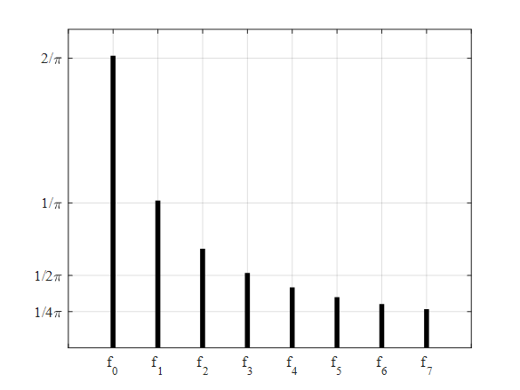
Interpretation: The above plot shows the amplitude plot for the sawtooth wave as shown in the figure provided.

Use the following MATLAB file can be used to construct the phase plot.

function Code_97924_19_6P_b()

for k = 1: 8

f(k) = k;

% define the phase

P(k) = (-1)^k*(pi/2);

end

% plot the values thus obtained

stem(f,P,'filled','LineWidth',4,'Color','k','Marker', 'none');

% define geometric properties

set(gca,'XTickLabel',{' ' 'f_0' 'f_1' 'f_2' 'f_3' 'f_4' 'f_5' 'f_6' 'f_7'});

set(gca,'YTick',[-pi -pi/2 0 pi/2 pi]);

set(gca,'YTickLabel',{'-\pi' '-\pi/2' '0' '\pi/2' '\pi'});

set(gca,'Fontname','Times New Roman','FontSize',12);

xlim([0, 9]); grid on

ylim([-pi-0.1, pi+0.1]); grid on

end

Execute the above code to obtain the plot as,

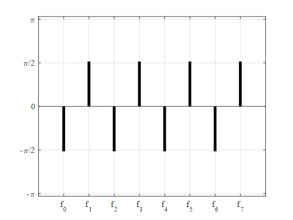
Interpretation: The above plot shows the phase line spectra for the sawtooth wave as shown in the figure provided.