
Concept explainers
Videos
A process engineer is considering two sampling plans. In the first, a sample of 10 will be selected and the lot accepted if 3 or fewer are found defective. In the second, the
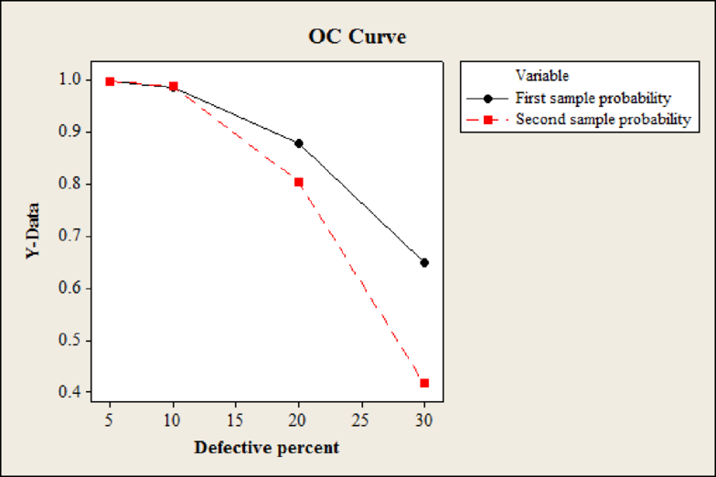
Develop the OC curve for each to compare the probability of acceptance for lots that are 5, 10, 20, and 30% defective.
Explain which of the plans would be recommend if you were the supplier.
Answer to Problem 31CE
Output using MINITAB software is given below:
Explanation of Solution
Calculation:
Let x denotes the accepting lots.
First sampling plan:
For 5% defective:
The probability of accepting lots that is 5% defective is,
Compute the probability value for x less than or equal to 3 using MINITAB.
Step by step procedure to obtain probability using MINITAB software is given as,
- Choose Calc > Probability Distributions > Binomial Distribution.
- Choose Cumulative probability.
- Enter Number of trials as 10 and Event probability as 0.05.
- In Input constant, enter 3.
- Click OK.
Output using MINITAB software is given below:
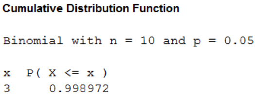
From the MINITAB output, the probability value is 0.999. That is,
For 10% defective:
The probability of accepting lots that is 10% defective is,
Compute the probability value for x less than or equal to 3 using MINITAB.
Step by step procedure to obtain probability using MINITAB software is given as,
- Choose Calc > Probability Distributions > Binomial Distribution.
- Choose Cumulative probability.
- Enter Number of trials as 10 and Event probability as 0.10.
- In Input constant, enter 3.
- Click OK.
Output using MINITAB software is given below:
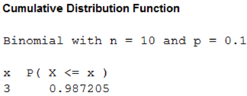
From the MINITAB output, the probability value is 0.987. That is,
For 20% defective:
The probability of accepting lots that is 20% defective is,
Compute the probability value for x less than or equal to 3 using MINITAB.
Step by step procedure to obtain probability using MINITAB software is given as,
- Choose Calc > Probability Distributions > Binomial Distribution.
- Choose Cumulative probability.
- Enter Number of trials as 10 and Event probability as 0.20.
- In Input constant, enter 3.
- Click OK.
Output using MINITAB software is given below:
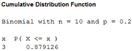
From the MINITAB output, the probability value is 0.879. That is,
For 30% defective:
The probability of accepting lots that is 30% defective is,
Compute the probability value for x less than or equal to 3 using MINITAB.
Step by step procedure to obtain probability using MINITAB software is given as,
- Choose Calc > Probability Distributions > Binomial Distribution.
- Choose Cumulative probability.
- Enter Number of trials as 10 and Event probability as 0.30.
- In Input constant, enter 3.
- Click OK.
Output using MINITAB software is given below:
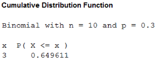
From the MINITAB output, the probability value is 0.649. That is,
The probability of accepting lots that are 5%, 10%, 20%, and 30% defective is,
| Defective Percent | Probability of acceptance |
| 5 | 0.999 |
| 10 | 0.987 |
| 20 | 0.879 |
| 30 | 0.649 |
Second sampling plan:
For 5% defective:
The probability of accepting lots that is 5% defective is,
Compute the probability value for x less than or equal to 5 using MINITAB.
Step by step procedure to obtain probability using MINITAB software is given as,
- Choose Calc > Probability Distributions > Binomial Distribution.
- Choose Cumulative probability.
- Enter Number of trials as 20 and Event probability as 0.05.
- In Input constant, enter 5.
- Click OK.
Output using MINITAB software is given below:
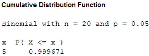
From the MINITAB output, the probability value is 0.999. That is,
For 10% defective:
The probability of accepting lots that is 10% defective is,
Compute the probability value for x less than or equal to 5 using MINITAB.
Step by step procedure to obtain probability using MINITAB software is given as,
- Choose Calc > Probability Distributions > Binomial Distribution.
- Choose Cumulative probability.
- Enter Number of trials as 20 and Event probability as 0.10.
- In Input constant, enter 5.
- Click OK.
Output using MINITAB software is given below:
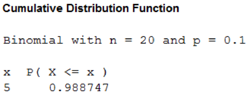
From the MINITAB output, the probability value is 0.988. That is,
For 20% defective:
The probability of accepting lots that is 20% defective is,
Compute the probability value for x less than or equal to 5 using MINITAB.
Step by step procedure to obtain probability using MINITAB software is given as,
- Choose Calc > Probability Distributions > Binomial Distribution.
- Choose Cumulative probability.
- Enter Number of trials as 20 and Event probability as 0.20.
- In Input constant, enter 5.
- Click OK.
Output using MINITAB software is given below:
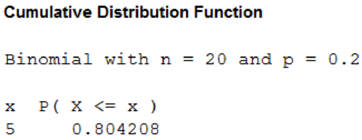
From the MINITAB output, the probability value is 0.804. That is,
For 30% defective:
The probability of accepting lots that is 30% defective is,
Compute the probability value for x less than or equal to 5 using MINITAB.
Step by step procedure to obtain probability using MINITAB software is given as,
- Choose Calc > Probability Distributions > Binomial Distribution.
- Choose Cumulative probability.
- Enter Number of trials as 20 and Event probability as 0.30.
- In Input constant, enter 5.
- Click OK.
Output using MINITAB software is given below:
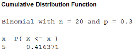
From the MINITAB output, the probability value is 0.416. That is,
The probability of accepting lots that are 5%, 10%, 20%, and 30% defective is,
| Defective Percent | Probability of acceptance |
| 5 | 0.999 |
| 10 | 0.988 |
| 20 | 0.804 |
| 30 | 0.416 |
Step by step procedure to obtain OC curve using MINITAB software is given as,
- Choose Graph > Scatterplot > select With Connect Line.
- In Y variable enter the column First sample probability.
- In X variable enter the column Defective percent.
- In Y variable enter the column Second sample probability.
- In X variable enter the column Defective percent.
- Select Multiple Graphs.
- Mark on Overlaid on the same graph under Show pairs of graph varibales.
- Click OK.
From the output, the black line represents the operating characteristic curve for the first plan and the red line represents the operating characteristic curve for the second plan. The probability of acceptance is more for first plan when compared with second plan because the probability line is above the probability line of second plan.
Since the probability of acceptance is higher for the first plan, the supplier should prefer first plan. But, it the supplier also takes the quality into account then supplier would prefer second plan because the percentage of defects is very low when compared to first plan.
Want to see more full solutions like this?
Chapter 19 Solutions
Loose Leaf for Statistical Techniques in Business and Economics


- 21. ANALYSIS OF LAST DIGITS Heights of statistics students were obtained by the author as part of an experiment conducted for class. The last digits of those heights are listed below. Construct a frequency distribution with 10 classes. Based on the distribution, do the heights appear to be reported or actually measured? Does there appear to be a gap in the frequencies and, if so, how might that gap be explained? What do you know about the accuracy of the results? 3 4 555 0 0 0 0 0 0 0 0 0 1 1 23 3 5 5 5 5 5 5 5 5 5 5 5 5 6 6 8 8 8 9arrow_forwardA side view of a recycling bin lid is diagramed below where two panels come together at a right angle. 45 in 24 in Width? — Given this information, how wide is the recycling bin in inches?arrow_forward1 No. 2 3 4 Binomial Prob. X n P Answer 5 6 4 7 8 9 10 12345678 8 3 4 2 2552 10 0.7 0.233 0.3 0.132 7 0.6 0.290 20 0.02 0.053 150 1000 0.15 0.035 8 7 10 0.7 0.383 11 9 3 5 0.3 0.132 12 10 4 7 0.6 0.290 13 Poisson Probability 14 X lambda Answer 18 4 19 20 21 22 23 9 15 16 17 3 1234567829 3 2 0.180 2 1.5 0.251 12 10 0.095 5 3 0.101 7 4 0.060 3 2 0.180 2 1.5 0.251 24 10 12 10 0.095arrow_forward
- step by step on Microssoft on how to put this in excel and the answers please Find binomial probability if: x = 8, n = 10, p = 0.7 x= 3, n=5, p = 0.3 x = 4, n=7, p = 0.6 Quality Control: A factory produces light bulbs with a 2% defect rate. If a random sample of 20 bulbs is tested, what is the probability that exactly 2 bulbs are defective? (hint: p=2% or 0.02; x =2, n=20; use the same logic for the following problems) Marketing Campaign: A marketing company sends out 1,000 promotional emails. The probability of any email being opened is 0.15. What is the probability that exactly 150 emails will be opened? (hint: total emails or n=1000, x =150) Customer Satisfaction: A survey shows that 70% of customers are satisfied with a new product. Out of 10 randomly selected customers, what is the probability that at least 8 are satisfied? (hint: One of the keyword in this question is “at least 8”, it is not “exactly 8”, the correct formula for this should be = 1- (binom.dist(7, 10, 0.7,…arrow_forwardKate, Luke, Mary and Nancy are sharing a cake. The cake had previously been divided into four slices (s1, s2, s3 and s4). What is an example of fair division of the cake S1 S2 S3 S4 Kate $4.00 $6.00 $6.00 $4.00 Luke $5.30 $5.00 $5.25 $5.45 Mary $4.25 $4.50 $3.50 $3.75 Nancy $6.00 $4.00 $4.00 $6.00arrow_forwardFaye cuts the sandwich in two fair shares to her. What is the first half s1arrow_forward
- Question 2. An American option on a stock has payoff given by F = f(St) when it is exercised at time t. We know that the function f is convex. A person claims that because of convexity, it is optimal to exercise at expiration T. Do you agree with them?arrow_forwardQuestion 4. We consider a CRR model with So == 5 and up and down factors u = 1.03 and d = 0.96. We consider the interest rate r = 4% (over one period). Is this a suitable CRR model? (Explain your answer.)arrow_forwardQuestion 3. We want to price a put option with strike price K and expiration T. Two financial advisors estimate the parameters with two different statistical methods: they obtain the same return rate μ, the same volatility σ, but the first advisor has interest r₁ and the second advisor has interest rate r2 (r1>r2). They both use a CRR model with the same number of periods to price the option. Which advisor will get the larger price? (Explain your answer.)arrow_forward
- Question 5. We consider a put option with strike price K and expiration T. This option is priced using a 1-period CRR model. We consider r > 0, and σ > 0 very large. What is the approximate price of the option? In other words, what is the limit of the price of the option as σ∞. (Briefly justify your answer.)arrow_forwardQuestion 6. You collect daily data for the stock of a company Z over the past 4 months (i.e. 80 days) and calculate the log-returns (yk)/(-1. You want to build a CRR model for the evolution of the stock. The expected value and standard deviation of the log-returns are y = 0.06 and Sy 0.1. The money market interest rate is r = 0.04. Determine the risk-neutral probability of the model.arrow_forwardSeveral markets (Japan, Switzerland) introduced negative interest rates on their money market. In this problem, we will consider an annual interest rate r < 0. We consider a stock modeled by an N-period CRR model where each period is 1 year (At = 1) and the up and down factors are u and d. (a) We consider an American put option with strike price K and expiration T. Prove that if <0, the optimal strategy is to wait until expiration T to exercise.arrow_forward
 Holt Mcdougal Larson Pre-algebra: Student Edition...AlgebraISBN:9780547587776Author:HOLT MCDOUGALPublisher:HOLT MCDOUGAL
 Big Ideas Math A Bridge To Success Algebra 1: Stu...AlgebraISBN:9781680331141Author:HOUGHTON MIFFLIN HARCOURTPublisher:Houghton Mifflin Harcourt
 Glencoe Algebra 1, Student Edition, 9780079039897...AlgebraISBN:9780079039897Author:CarterPublisher:McGraw Hill
 College Algebra (MindTap Course List)AlgebraISBN:9781305652231Author:R. David Gustafson, Jeff HughesPublisher:Cengage Learning
