
(a)
To explain: The process of simulating the roll of one balanced die as well as a roll of two balanced dice.
(a)
Answer to Problem 23E
Solution: To simulate the result of rolling of single die, one-digit random number is between 1 and 6 that is selected from the random number table. By repeating the above-mentioned process for two times and adding the outcomes of the two rolls, the result of the roll of two balanced die is obtained.
Explanation of Solution
The result of the roll of two dice can be obtained by simulation. For that the outcome of individual die is obtained by repeating the above-mentioned process. Then the outcomes of the two rolls are added to obtain the result of the roll of two balanced die.
(b)
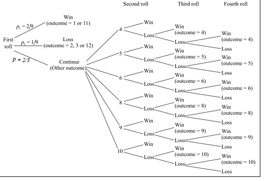
To graph: The tree diagram where the
(b)
Explanation of Solution
Calculation:
If the combinations
The probability of getting a 7 or 11 is calculated as follows:
If the outcomes are 2, 3, or 12, the player loses. The cases where the player will lose are
The players can repeat the game if other outcomes come. The player will continue the game until he wins with repeating the first outcomes or loses by rolling a 7. The probabilities that the player will get other outcomes will be calculated as follows:
That is, the probability of occurrence of any of the outcomes among 4, 5, 6, 8, 9, or 10 is
Graph: The tree diagram is drawn starting from the first roll. Each of the outcomes has different probability of occurrence in each step. The tree diagram is shown below:
To estimate the probability, the process of simulation that is described in part (a) is used. The one-digit random numbers are chosen from the random number table, Table A, starting from the 114th row and the 1st column of the table. The random number is selected between 1 and 6. If the selected number is more than 6 or equal to 0, then that number is rejected. First 20 numbers are selected as outcomes of the one die and the next 20 numbers indicates the outcomes of second die. The numbers are selected for 20 repetitions.
The selected numbers and the results are shown in the below table:
| Repetition | Die 1 | Die 2 | Result |
| 1 | 4 | 1 | 5 |
| 2 | 5 | 5 | 10 |
| 3 | 1 | 6 | 7 |
| 4 | 4 | 1 | 5 |
| 5 | 3 | 4 | 7 |
| 6 | 2 | 1 | 3 |
| 7 | 2 | 6 | 8 |
| 8 | 5 | 4 | 9 |
| 9 | 3 | 4 | 7 |
| 10 | 6 | 3 | 9 |
| 11 | 6 | 2 | 8 |
| 12 | 2 | 2 | 4 |
| 13 | 3 | 2 | 5 |
| 14 | 1 | 4 | 5 |
| 15 | 5 | 3 | 8 |
| 16 | 6 | 6 | 12 |
| 17 | 2 | 1 | 3 |
| 18 | 2 | 4 | 6 |
| 19 | 2 | 5 | 7 |
| 20 | 3 | 2 | 5 |
There are 4 cases where the player wins in the first roll among 20 repetitions. Therefore, the required probability is calculated as follows:
Interpretation: There is 20% chance that the player wins the game in first roll.
Want to see more full solutions like this?
Chapter 19 Solutions
Statistics: Concepts and Controversies - WebAssign and eBook Access

- Harvard University California Institute of Technology Massachusetts Institute of Technology Stanford University Princeton University University of Cambridge University of Oxford University of California, Berkeley Imperial College London Yale University University of California, Los Angeles University of Chicago Johns Hopkins University Cornell University ETH Zurich University of Michigan University of Toronto Columbia University University of Pennsylvania Carnegie Mellon University University of Hong Kong University College London University of Washington Duke University Northwestern University University of Tokyo Georgia Institute of Technology Pohang University of Science and Technology University of California, Santa Barbara University of British Columbia University of North Carolina at Chapel Hill University of California, San Diego University of Illinois at Urbana-Champaign National University of Singapore McGill…arrow_forwardName Harvard University California Institute of Technology Massachusetts Institute of Technology Stanford University Princeton University University of Cambridge University of Oxford University of California, Berkeley Imperial College London Yale University University of California, Los Angeles University of Chicago Johns Hopkins University Cornell University ETH Zurich University of Michigan University of Toronto Columbia University University of Pennsylvania Carnegie Mellon University University of Hong Kong University College London University of Washington Duke University Northwestern University University of Tokyo Georgia Institute of Technology Pohang University of Science and Technology University of California, Santa Barbara University of British Columbia University of North Carolina at Chapel Hill University of California, San Diego University of Illinois at Urbana-Champaign National University of Singapore…arrow_forwardA company found that the daily sales revenue of its flagship product follows a normal distribution with a mean of $4500 and a standard deviation of $450. The company defines a "high-sales day" that is, any day with sales exceeding $4800. please provide a step by step on how to get the answers in excel Q: What percentage of days can the company expect to have "high-sales days" or sales greater than $4800? Q: What is the sales revenue threshold for the bottom 10% of days? (please note that 10% refers to the probability/area under bell curve towards the lower tail of bell curve) Provide answers in the yellow cellsarrow_forward
- Find the critical value for a left-tailed test using the F distribution with a 0.025, degrees of freedom in the numerator=12, and degrees of freedom in the denominator = 50. A portion of the table of critical values of the F-distribution is provided. Click the icon to view the partial table of critical values of the F-distribution. What is the critical value? (Round to two decimal places as needed.)arrow_forwardA retail store manager claims that the average daily sales of the store are $1,500. You aim to test whether the actual average daily sales differ significantly from this claimed value. You can provide your answer by inserting a text box and the answer must include: Null hypothesis, Alternative hypothesis, Show answer (output table/summary table), and Conclusion based on the P value. Showing the calculation is a must. If calculation is missing,so please provide a step by step on the answers Numerical answers in the yellow cellsarrow_forwardShow all workarrow_forward
 MATLAB: An Introduction with ApplicationsStatisticsISBN:9781119256830Author:Amos GilatPublisher:John Wiley & Sons Inc
 Probability and Statistics for Engineering and th...StatisticsISBN:9781305251809Author:Jay L. DevorePublisher:Cengage Learning
 Statistics for The Behavioral Sciences (MindTap C...StatisticsISBN:9781305504912Author:Frederick J Gravetter, Larry B. WallnauPublisher:Cengage Learning
 Elementary Statistics: Picturing the World (7th E...StatisticsISBN:9780134683416Author:Ron Larson, Betsy FarberPublisher:PEARSON
 The Basic Practice of StatisticsStatisticsISBN:9781319042578Author:David S. Moore, William I. Notz, Michael A. FlignerPublisher:W. H. Freeman
 Introduction to the Practice of StatisticsStatisticsISBN:9781319013387Author:David S. Moore, George P. McCabe, Bruce A. CraigPublisher:W. H. Freeman