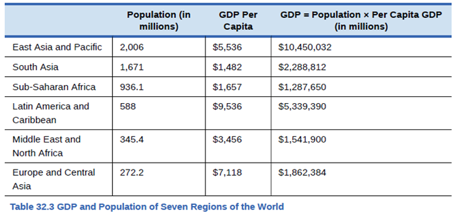
Using the data in Table 32.3, rank the seven regions of the world according to GDP and then according to GDP per capita.
The rank:
The given regions of the world according to the GDP and then according to the GDP per capita
Explanation of Solution
As per the table given, the rankings are as follows:
| Countries | Population
|
GDP per capita
|
Ranking as GDP | |
| East Asia and Pacific | I | |||
| Latin America and Caribbean | II | |||
| South Asia | III | |||
| Europe and Central Asia | IV | |||
| Middle East and North Africa | V | |||
| Sub-Saharan Asia | VI |
| Countries | Population
|
GDP per capita
|
Ranking as GDP per capita | |
| Latin America and Caribbean | I | |||
| Europe and Central Asia | II | |||
| East Asia and Pacific | III | |||
| Middle East and North Africa | IV | |||
| Sub-Saharan Asia | V | |||
| South Asia | VI |
Economist measures a nation’s standard of living through its GDP per capita. GDP measures annual economic output that is total value of goods and services produced within a country.
The low-income countries are those which are having GDP per capita income less than
Want to see more full solutions like this?
Chapter 19 Solutions
Principles of Macroeconomics 2e
Additional Business Textbook Solutions
Horngren's Financial & Managerial Accounting, The Financial Chapters (Book & Access Card)
Gitman: Principl Manageri Finance_15 (15th Edition) (What's New in Finance)
Foundations Of Finance
MARKETING:REAL PEOPLE,REAL CHOICES
Corporate Finance (4th Edition) (Pearson Series in Finance) - Standalone book
Horngren's Accounting (12th Edition)

- In a small open economy with a floating exchange rate, the supply of real money balances is fixed and a rise in government spending ______ Group of answer choices Raises the interest rate so that net exports must fall to maintain equilibrium in the goods market. Cannot change the interest rate so that net exports must fall to maintain equilibrium in the goods market. Cannot change the interest rate so income must rise to maintain equilibrium in the money market Raises the interest rate, so that income must rise to maintain equilibrium in the money market.arrow_forwardSuppose a country with a fixed exchange rate decides to implement a devaluation of its currency and commits to maintaining the new fixed parity. This implies (A) ______________ in the demand for its goods and a monetary (B) _______________. Group of answer choices (A) expansion ; (B) contraction (A) contraction ; (B) expansion (A) expansion ; (B) expansion (A) contraction ; (B) contractionarrow_forwardAssume a small open country under fixed exchanges rate and full capital mobility. Prices are fixed in the short run and equilibrium is given initially at point A. An exogenous increase in public spending shifts the IS curve to IS'. Which of the following statements is true? Group of answer choices A new equilibrium is reached at point B. The TR curve will shift down until it passes through point B. A new equilibrium is reached at point C. Point B can only be reached in the absence of capital mobility.arrow_forward
- A decrease in money demand causes the real interest rate to _____ and output to _____ in the short run, before prices adjust to restore equilibrium. Group of answer choices rise; rise fall; fall fall; rise rise; fallarrow_forwardIf a country's policy makers were to continously use expansionary monetary policy in an attempt to hold unemployment below the natural rate , the long urn result would be? Group of answer choices a decrease in the unemployment rate an increase in the level of output All of these an increase in the rate of inflationarrow_forwardA shift in the Aggregate Supply curve to the right will result in a move to a point that is southwest of where the economy is currently at. Group of answer choices True Falsearrow_forward
- An oil shock can cause stagflation, a period of higher inflation and higher unemployment. When this happens, the economy moves to a point to the northeast of where it currently is. After the economy has moved to the northeast, the Federal Reserve can reduce that inflation without having to worry about causing more unemployment. Group of answer choices True Falsearrow_forwardThe long-run Phillips Curve is vertical which indicates Group of answer choices that in the long-run, there is no tradeoff between inflation and unemployment. that in the long-run, there is no tradeoff between inflation and the price level. None of these that in the long-run, the economy returns to a 4 percent level of inflation.arrow_forwardSuppose the exchange rate between the British pound and the U.S. dollar is £1 = $2.00. The U.S. government implementsU.S. government implements a contractionary fiscal policya contractionary fiscal policy. Illustrate the impact of this change in the market for pounds. 1.) Using the line drawing tool, draw and label a new demand line. 2.) Using the line drawing tool, draw and label a new supply line. Note: Carefully follow the instructions above and only draw the required objects.arrow_forward
- Just Part D please, this is for environmental economicsarrow_forward3. Consider a single firm that manufactures chemicals and generates pollution through its emissions E. Researchers have estimated the MDF and MAC curves for the emissions to be the following: MDF = 4E and MAC = 125 – E Policymakers have decided to implement an emissions tax to control pollution. They are aware that a constant per-unit tax of $100 is an efficient policy. Yet they are also aware that this policy is not politically feasible because of the large tax burden it places on the firm. As a result, policymakers propose a two- part tax: a per unit tax of $75 for the first 15 units of emissions an increase in the per unit tax to $100 for all further units of emissions With an emissions tax, what is the general condition that determines how much pollution the regulated party will emit? What is the efficient level of emissions given the above MDF and MAC curves? What are the firm's total tax payments under the constant $100 per-unit tax? What is the firm's total cost of compliance…arrow_forward2. Answer the following questions as they relate to a fishery: Why is the maximum sustainable yield not necessarily the optimal sustainable yield? Does the same intuition apply to Nathaniel's decision of when to cut his trees? What condition will hold at the equilibrium level of fishing in an open-access fishery? Use a graph to explain your answer, and show the level of fishing effort. Would this same condition hold if there was only one boat in the fishery? If not, what condition will hold, and why is it different? Use the same graph to show the single boat's level of effort. Suppose you are given authority to solve the open-access problem in the fishery. What is the key problem that you must address with your policy?arrow_forward


 Principles of Economics 2eEconomicsISBN:9781947172364Author:Steven A. Greenlaw; David ShapiroPublisher:OpenStax
 Economics (MindTap Course List)EconomicsISBN:9781337617383Author:Roger A. ArnoldPublisher:Cengage Learning