Chapter 19, Problem 1PA

(a)

To determine

Consumption and saving.

Explanation of Solution

According to the life-cycle model of consumption, the consumption of an individual depends on the income earned in the entire life time of an individual.

The total life time income of the individuals can be calculated as the sum of income they earn in different periods using Equation (1) as follows:

$\text{Life-time income}={\text{Income}}_1+{\text{Income}}_2+\mathrm{...}+{\text{Income}}_{\text{n}}$ (1)

Given that A enjoys $100,000 in three periods and F enjoys $40,000 in period1, $100,000 in period2, and $160,000 in period3, both individuals consume for 5 periods in life.

The life-time income of A can be calculated by substituting the respective values in Equation (1) as follows:

$\begin{array}{c}{\text{Life-time income}}_{\text{A}}=100,000+100,000+100,000\\ =300,000\end{array}$

Thus, the life-time income of A is $300,000.

The life-time income of F can be calculated by substituting the respective values in Equation (1) as follows:

$\begin{array}{c}{\text{Life-time income}}_{\text{F}}=40,000+100,000+160,000\\ =300,000\end{array}$

Thus, the life-time income of F is $300,000.

The life-time consumption of individuals can be calculated using Equation (2) as follows:

$\text{Life-time consumption}=\frac{\text{Life-time income}}{\text{Number of periods}}$ (2)

The life-time consumption of A can be calculated by substituting the respective values in Equation (2) as follows:

$\begin{array}{c}{\text{Life-time consumption}}_{\text{A}}=\frac{\text{300,000}}{\text{5}}\\ =60,000\end{array}$

The life-time consumption of A is $60,000.

The life-time consumption of F can be calculated by substituting the respective values in Equation (2) as follows:

$\begin{array}{c}{\text{Life-time consumption}}_{\text{F}}=\frac{\text{300,000}}{\text{5}}\\ =60,000\end{array}$

The life-time consumption of F is $60,000.

The savings can be calculated as the part of income, which is not consumed. The savings can be calculated using Equation (3) as follows:

$\text{Saving}=\text{Income}-\text{Consumption}$ (3)

The saving in period 1 for A can be calculated by substituting the respective value in Equation (3) as follows:

$\begin{array}{c}{\text{Saving}}_1={\text{Income}}_1-{\text{Consumption}}_1\\ =100,000-60,000\\ =40,000\end{array}$

Thus, A’ savings for period 1 is $40,000.

Table 1 shows the values of savings for A and F in different periods calculated using Equations 1, 2, and 3.

Table 1

	A	F
S1	40,000	-20,000
S2	40,000	40,000
S3	40,000	100,000
S4	-60,000	-60,000
S5	-60,000	-60,000

Economics Concept Introduction

Life-cycle theory: Life-cycle theory developed by Franco Modigliani and Richard Brumberg relates the spending and saving habits of an individual to the course of their life time.

Savings: Savings is defined as that part of income that is not consumed in the current period and is to be used for future consumption.

(b)

To determine

The wealth of individuals.

Explanation of Solution

The wealth of an individual is calculated as the accumulated saving in each period.

The wealth can be calculated using Equation (4) as follows:

${\text{Wealth}}_{\text{n}}={\text{Saving}}_0+{\text{Saving}}_1+\mathrm{...}+{\text{Saving}}_{\text{n}}$ (4)

The wealth of individual A in the beginning of period 2 is calculated by substituting the respective values in Equation (4) as follows:

$\begin{array}{c}{\text{Wealth}}_{\text{A}}={\text{Saving}}_0+{\text{Saving}}_1\\ =0+40,000\\ =40,000\end{array}$

Thus, the wealth of A in the beginning of period 2 is $40,000.

Table 2 shows the values of wealth for A and F in different periods, which are calculated using Equation 4.

Table 1

	A	F
W1	0	0
W2	40,000	-20,000
W3	80,000	20,000
W4	120,000	120,000
W5	60,000	60,000
W6	0	0

It is evident from the table values that there is no wealth in period1 and period 6.

(c)

To determine

The graphical representation of consumption, income, and wealth of the individuals.

Explanation of Solution

Figure 1 given below shows the consumption, income, and wealth of A.

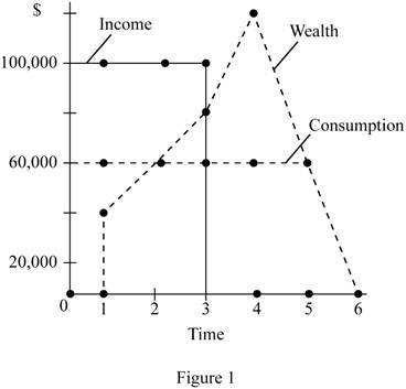
The horizontal axis of Figure 1 measures the time period, and the vertical axis measures the consumption, income, and wealth. A enjoys a fixed income over the first 3 periods, and hence he also has a constant pattern of consumption as clearly depicted in Figure 1. A saves a part of his income and thus gradually increases his wealth during his earning years and gradually dissaves when he leads his retirement life. His pattern of consumption, income, and wealth is according to the prediction of the life-cycle model.

Figure 2 given below shows the consumption, income, and wealth of F.

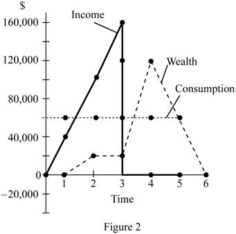
The horizontal axis of Figure 1 measures the time period, and the vertical axis measures the consumption, income, and wealth. F increases his income gradually, and this would force him to borrow initially to enjoy a smooth consumption. When his income increases, he would accumulate wealth and then use it for his consumption in the retirement life.

Economics Concept Introduction

Savings: Savings is defined as that part of income that is not consumed in the current period and is to be used for future consumption.

Dissaving: The act of spending more than earned in the current period or spending the past savings is known as dissaving.

(d)

To determine

The impact of borrowing.

Explanation of Solution

A has fixed income from the initial years of earning, and hence there is no need for him to borrow. Thus, A’s consumption or income will not be affected when there is a borrowing constraint. However, F depends on borrowing for his initial period. When there is a borrowing constraint, F has to spend his entire income of $40,000 in the initial period. For the later periods, he smooths his consumption by dividing the lifetime income across the remaining periods.

The life-time income of F can be calculated by substituting the respective values in Equation (1) as follows:

$\begin{array}{c}{\text{Life-time income}}_{\text{F}}=100,000+160,000\\ =260,000\end{array}$

Thus, the life-time income of F is $260,000.

The life-time consumption of F can be calculated by substituting the respective values in Equation (2) as follows:

$\begin{array}{c}{\text{Life-time consumption}}_{\text{F}}=\frac{\text{260,000}}{4}\\ =65,000\end{array}$

The life-time consumption of F is $65,000.

The saving in period 2 for F can be calculated by substituting the respective values in Equation (3) as follows:

$\begin{array}{c}{\text{Saving}}_2={\text{Income}}_2-{\text{Consumption}}_2\\ =100,000-65,000\\ =35,000\end{array}$

Thus, F’s savings for period 2 is $35,000.

The wealth of individual F in the beginning of period 2 is calculated by substituting the respective values in Equation (4) as follows:

$\begin{array}{c}{\text{Wealth}}_{\text{F}}={\text{Saving}}_0+{\text{Saving}}_1\\ =0+0\\ =0\end{array}$

Thus, the wealth of A in the beginning of period 2 is $40,000.

Table 2 shows the values of savings and wealth F in different periods, which are calculated using Equations 3 and 4.

Table 1

Period	F's Consumption	F's Savings	F's Wealth
0	0	0	0
1	40,000	0	0
2	65,000	35,000	35,000
3	65,000	95,000	130,000
4	65,000	-65,000	65,000
5	65,000	-65,000	0

Figure 3 given below shows the consumption, income, and wealth of F.

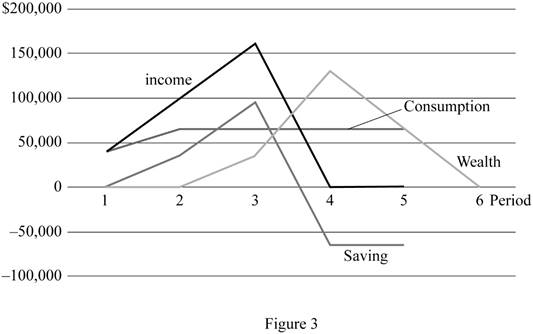
The horizontal axis of Figure 1 measures the time period, and the vertical axis measures the consumption, income, and wealth. F increases his income gradually. However, he faces borrowing constraints, and hence he can only use his initial income for consumption. When his income increases, he would accumulate wealth, and then use it for his consumption in the retirement life.

Economics Concept Introduction

Savings: Savings is defined as that part of income that is not consumed in the current period and is to be used for future consumption.

Dissaving: The act of spending more than earned in the current period or spending the past savings is known as dissaving.