Concept explainers
a)
To solve: The linear programming problem and answer the given questions.
Introduction:
Linear programming:
Linear programming is a mathematical modelling method where a linear function is maximized or minimized taking into consideration the various constraints present in the problem. It is useful in making quantitative decisions in business planning.
a)
Explanation of Solution
Given information:
Calculation of coordinates for each constraint and objective function:
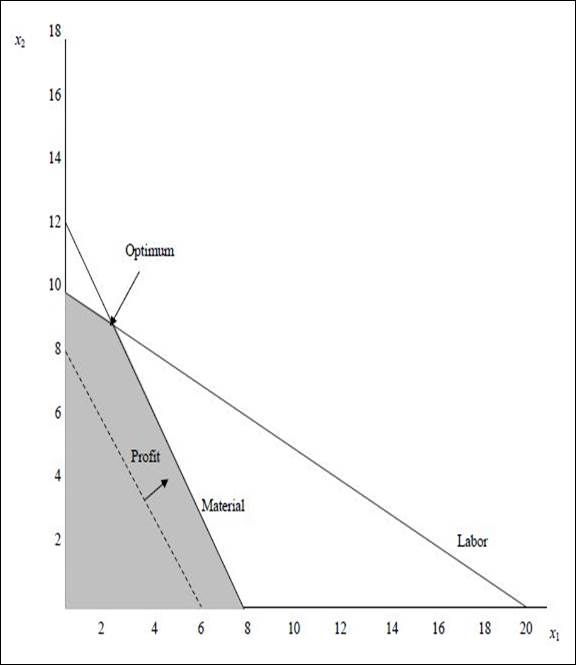
Constraint 1:
Constraint 2:
Objective function:
The problem is solved with iso-profit line method.
Graph:
(1) Optimal value of the decision variables and Z:
The coordinates for the profit line is (6, 8). The profit line is moved away from the origin. The highest point at which the profit line intersects in the feasible region will be the optimum solution. The following equation are solved as simultaneous equation to find optimum solution.
Solving (1)and (2)we get,
The values are substituted in the objective function to find the objective function value.
Optimal solution:
(2)
None of the constraints are having slack. Both the ≤ constraints are binding.
(3)
There are no ≥ constraints. Hence, none of the constraints have surplus.
(4)
There are no redundant constraints.
b)
To solve: The linear programming problem and answer the questions.
Introduction:
Linear programming:
Linear programming is a mathematical modelling method where a linear function is maximized or minimized taking into consideration the various constraints present in the problem. It is useful in making quantitative decisions in business planning.
b)
Explanation of Solution
Given information:
Calculation of coordinates for each constraint and objective function:
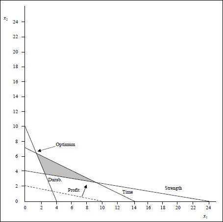
Constraint 1:
Constraint 2:
Constraint 3:
Objective function:
The problem is solved with iso-profit line method.
Graph:
(1) Optimal value of the decision variables and Z:
The coordinates for the profit line is (10, 2). The profit line is moved away from the origin. The highest point at which the profit line intersects in the feasible region will be the optimum solution. The following equations are solved as simultaneous equation to find optimum solution.
Solving (1)and (2)we get,
The values are substituted in the objective function to find the objective function value.
Optimal solution:
(2)
None of the constraints are having slack. The time constraint has ≤ and it is binding.
(3)
Durability and strength constraints have ≥ in them. The durability constraint is binding and has no surplus. The strength constraint has surplus as shown below:
The surplus is 15 (39 -24).
(4)
There are no redundant constraints.
c)
To solve: The linear programming problem and answer the questions.
Introduction:
Linear programming:
Linear programming is a mathematical modelling method where a linear function is maximized or minimized taking into consideration the various constraints present in the problem. It is useful in making quantitative decisions in business planning.
c)
Explanation of Solution
Given information:
Calculation of coordinates for each constraint and objective function:
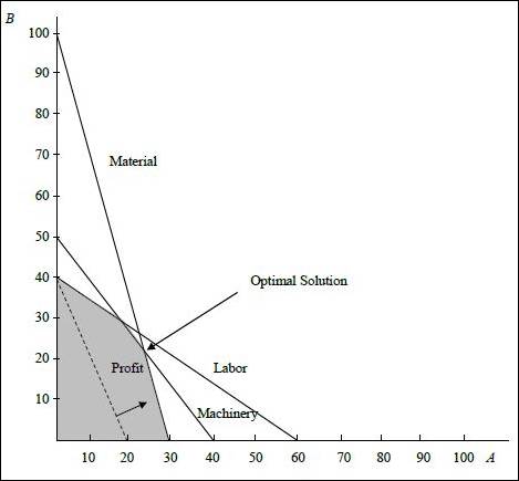
Constraint 1:
Constraint 2:
Constraint 3:
Objective function:
The problem is solved with iso-profit line method.
Graph:
(1) Optimal value of the decision variables and Z:
The coordinates for the profit line is (20, 40). The profit line is moved away from the origin. The highest point at which the profit line intersects in the feasible region will be the optimum solution. The following equation are solved as simultaneous equation to find optimum solution.
Solving (1) and (2) we get,
The values are substituted in the objective function to find the objective function value.
Optimal solution:
(2)
The material and machinery constraint has ≤ and it is binding and has zero slack. The labor constraint has slack as shown below:
The slack is 120 (1,200 – 1,080).
(3)
There are no constraints with ≥. Hence, no constraints have surplus.
(4)
There are no redundant constraints
Want to see more full solutions like this?
Chapter 19 Solutions
OPERATIONS MANAGEMENT(LL)-W/CONNECT


- The Donald Fertilizer Company produces industrial chemical fertilizers. The projected manufacturing requirements (in gallons) for the next four quarters are 60,000, 90,000, 90,000, and 140,000 respectively. A level workforce is desired, relying only on anticipation inventory as a supply option. Stockouts and backorders are to be avoided, as are overtime and undertime. a. Determine the quarterly production rate required to meet total demand for the year, and minimize the anticipation inventory that would be left over at the end of the year. Beginning inventory is 0. The quarterly production rate is ☐ gallons. (Enter your response as an integer.)arrow_forwardHow would you design an operations plan and schedule for a new product/service? What factors would you consider and what challenges would you anticipate? Why are these factors and challenges relevant and how would you address them?arrow_forwardYou are the newly appointed CEO of TechSouth, a South African multinational technology company based in Cape Town. TechSouth specialises in manufacturing smartphones, laptops, and smart home devices. The company has a significant presence in the African market and has recently expanded into Europe and Asia. However, TechSouth is facing several critical challenges:· Declining Market Share - Over the past three years, TechSouth has lost considerable market share to both localcompetitors and international giants like Samsung and Apple. The company's products are perceived as outdated and lacking innovation.· Employee Engagement Issues - Recent employee surveys indicate low morale and engagement levels, particularly among the younger workforce, leading to high turnover rates. Many employees feel disconnected from the company's vision and mission.· Siloed Departments - The organizational structure at TechSouth is highly siloed, with departments operatingindependently rather than…arrow_forward
- What is the best way to manage emotions and thoughts? How to work through Emotions and thoughts?arrow_forwardWhat are the emotions or stressful thoughts? What are the differences between them? How can we work through the emotions or stressful thoughts? How can we avoid or prevent emotions or stressful thoughts from happening or occurring? What are the obstacles?arrow_forwardMain Challenges at TechInnovateStrategic DirectionTechInnovate's board of directors is pushing for a more aggressive expansion into emerging markets, particularly in Africaand Southeast Asia. However, there's internal disagreement about whether to focus on these new markets or consolidatetheir position in existing ones. Sarah Chen favors rapid expansion, while some senior executives advocate for a morecautious approach.Ethical ConcernsThe company's AI algorithms have come under scrutiny for potential biases, particularly in facial recognition technology.There are concerns that these biases disproportionately affect minority groups. Some employees have voiced ethicalconcerns about selling this technology to law enforcement agencies without addressing these issues.Team Leadership and DiversityTechInnovate's leadership team is predominantly male and Western, despite its global presence. There's growing pressurefrom employees and some board members to diversify the leadership team to…arrow_forward
- Sarah Anderson, the Marketing Manager at Exeter Township's Cultural Center, is conducting research on the attendance history for cultural events in the area over the past ten years. The following data has been collected on the number of attendees who registered for events at the cultural center. Year Number of Attendees 1 700 2 248 3 633 4 458 5 1410 6 1588 7 1629 8 1301 9 1455 10 1989 You have been hired as a consultant to assist in implementing a forecasting system that utilizes various forecasting techniques to predict attendance for Year 11. a) Calculate the Three-Period Simple Moving Average b) Calculate the Three-Period Weighted Moving Average (weights: 50%, 30%, and 20%; use 50% for the most recent period, 30% for the next most recent, and 20% for the oldest) c) Apply Exponential Smoothing with the smoothing constant alpha = 0.2. d) Perform a Simple Linear Regression analysis and provide the adjusted…arrow_forwardRuby-Star Incorporated is considering two different vendors for one of its top-selling products which has an average weekly demand of 70 units and is valued at $90 per unit. Inbound shipments from vendor 1 will average 390 units with an average lead time (including ordering delays and transit time) of 4 weeks. Inbound shipments from vendor 2 will average 490 units with an average lead time of 2 weeksweeks. Ruby-Star operates 52 weeks per year; it carries a 4-week supply of inventory as safety stock and no anticipation inventory. Part 2 a. The average aggregate inventory value of the product if Ruby-Star used vendor 1 exclusively is $enter your response here.arrow_forwardSam's Pet Hotel operates 50 weeks per year, 6 days per week, and uses a continuous review inventory system. It purchases kitty litter for $13.00 per bag. The following information is available about these bags: > Demand 75 bags/week > Order cost = $52.00/order > Annual holding cost = 20 percent of cost > Desired cycle-service level = 80 percent >Lead time = 5 weeks (30 working days) > Standard deviation of weekly demand = 15 bags > Current on-hand inventory is 320 bags, with no open orders or backorders. a. Suppose that the weekly demand forecast of 75 bags is incorrect and actual demand averages only 50 bags per week. How much higher will total costs be, owing to the distorted EOQ caused by this forecast error? The costs will be $higher owing to the error in EOQ. (Enter your response rounded to two decimal places.)arrow_forward
- Yellow Press, Inc., buys paper in 1,500-pound rolls for printing. Annual demand is 2,250 rolls. The cost per roll is $625, and the annual holding cost is 20 percent of the cost. Each order costs $75. a. How many rolls should Yellow Press order at a time? Yellow Press should order rolls at a time. (Enter your response rounded to the nearest whole number.)arrow_forwardPlease help with only the one I circled! I solved the others :)arrow_forwardOsprey Sports stocks everything that a musky fisherman could want in the Great North Woods. A particular musky lure has been very popular with local fishermen as well as those who buy lures on the Internet from Osprey Sports. The cost to place orders with the supplier is $40/order; the demand averages 3 lures per day, with a standard deviation of 1 lure; and the inventory holding cost is $1.00/lure/year. The lead time form the supplier is 10 days, with a standard deviation of 2 days. It is important to maintain a 97 percent cycle-service level to properly balance service with inventory holding costs. Osprey Sports is open 350 days a year to allow the owners the opportunity to fish for muskies during the prime season. The owners want to use a continuous review inventory system for this item. Refer to the standard normal table for z-values. a. What order quantity should be used? lures. (Enter your response rounded to the nearest whole number.)arrow_forward
 Practical Management ScienceOperations ManagementISBN:9781337406659Author:WINSTON, Wayne L.Publisher:Cengage,