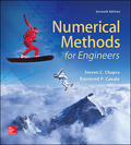
EBK NUMERICAL METHODS FOR ENGINEERS
7th Edition
ISBN: 8220100254147
Author: Chapra
Publisher: MCG
expand_more
expand_more
format_list_bulleted
Concept explainers
Textbook Question
Chapter 18, Problem 4P
Repeat Probs. 18.1 through 18.3 using the Lagrange polynomial.
Expert Solution & Answer
Want to see the full answer?
Check out a sample textbook solution
Students have asked these similar questions
Can you provide steps and an explaination on how the height value to calculate the Pressure at point B is (-5-3.5) and the solution is 86.4kPa.
PROBLEM 3.46
The solid cylindrical rod BC of length L = 600
mm is attached to the rigid lever AB of length a
= 380 mm and to the support at C. When a 500
N force P is applied at A, design specifications
require that the displacement of A not exceed
25 mm when a 500 N force P is applied at A
For the material indicated determine the
required diameter of the rod.
Aluminium: Tall = 65 MPa, G = 27 GPa.
A
Find the equivalent mass of the rocker arm assembly with respect to the x coordinate.
k₁
mi
m2
k₁
Chapter 18 Solutions
EBK NUMERICAL METHODS FOR ENGINEERS
Ch. 18 - 18.1 Estimate the common logarithm of 10 using...Ch. 18 - 18.2 Fit a second-order Newton’s interpolating...Ch. 18 - 18.3 Fit a third-order Newton’s interpolating...Ch. 18 - Repeat Probs. 18.1 through 18.3 using the Lagrange...Ch. 18 - 18.5 Given these...Ch. 18 - 18.6 Given these data
x 1 2 3 5 7 8
...Ch. 18 - Repeat Prob. 18.6 using Lagrange polynomials of...Ch. 18 - 18.8 The following data come from a table that was...Ch. 18 - 18.9 Use Newton’s interpolating polynomial to...Ch. 18 - Use Newtons interpolating polynomial to determine...
Ch. 18 - 18.11 Employ inverse interpolation using a cubic...Ch. 18 - 18.12 Employ inverse interpolation to determine...Ch. 18 - 18.13 Develop quadratic splines for the first five...Ch. 18 - 18.14 Develop cubic splines for the data in Prob....Ch. 18 - Determine the coefficients of the parabola that...Ch. 18 - Determine the coefficients of the cubic equation...Ch. 18 - 18.17 Develop, debug, and test a program in either...Ch. 18 - 18.18 Test the program you developed in Prob....Ch. 18 - 18.19 Use the program you developed in Prob. 18.17...Ch. 18 - Use the program you developed in Prob. 18.17 to...Ch. 18 - Develop, debug, and test a program in either a...Ch. 18 - 18.22 A useful application of Lagrange...Ch. 18 - Develop, debug, and test a program in either a...Ch. 18 - Use the software developed in Prob. 18.23 to fit...Ch. 18 - Use the portion of the given steam table for...Ch. 18 - The following is the built-in humps function that...Ch. 18 - 18.28 The following data define the sea-level...Ch. 18 - 18.29 Generate eight equally-spaced points from...Ch. 18 - 18.30 Temperatures are measured at various points...
Additional Engineering Textbook Solutions
Find more solutions based on key concepts
Is there a relationship between wine consumption and deaths from heart disease? The table gives data from 19 de...
College Algebra Essentials (5th Edition)
23. A plant nursery sells two sizes of oak trees to landscapers. Large trees cost the nursery $120 from the gro...
College Algebra (Collegiate Math)
CHECK POINT I Consider the six jokes about books by Groucho Marx. Bob Blitzer. Steven Wright, HennyYoungman. Je...
Thinking Mathematically (6th Edition)
NOTE: Write your answers using interval notation when appropriate.
CHECKING ANALYTIC SKILLS Fill in each blank ...
Graphical Approach To College Algebra
Let F be a continuous distribution function. If U is uniformly distributed on (0,1), find the distribution func...
A First Course in Probability (10th Edition)
The largest polynomial that divides evenly into a list of polynomials is called the _______.
Elementary & Intermediate Algebra
Knowledge Booster
Learn more about
Need a deep-dive on the concept behind this application? Look no further. Learn more about this topic, mechanical-engineering and related others by exploring similar questions and additional content below.Similar questions
- 2. Figure below shows a U-tube manometer open at both ends and containing a column of liquid mercury of length l and specific weight y. Considering a small displacement x of the manometer meniscus from its equilibrium position (or datum), determine the equivalent spring constant associated with the restoring force. Datum Area, Aarrow_forward1. The consequences of a head-on collision of two automobiles can be studied by considering the impact of the automobile on a barrier, as shown in figure below. Construct a mathematical model (i.e., draw the diagram) by considering the masses of the automobile body, engine, transmission, and suspension and the elasticity of the bumpers, radiator, sheet metal body, driveline, and engine mounts.arrow_forward3.) 15.40 – Collar B moves up at constant velocity vB = 1.5 m/s. Rod AB has length = 1.2 m. The incline is at angle = 25°. Compute an expression for the angular velocity of rod AB, ė and the velocity of end A of the rod (✓✓) as a function of v₂,1,0,0. Then compute numerical answers for ȧ & y_ with 0 = 50°.arrow_forward
- 2.) 15.12 The assembly shown consists of the straight rod ABC which passes through and is welded to the grectangular plate DEFH. The assembly rotates about the axis AC with a constant angular velocity of 9 rad/s. Knowing that the motion when viewed from C is counterclockwise, determine the velocity and acceleration of corner F.arrow_forward500 Q3: The attachment shown in Fig.3 is made of 1040 HR. The static force is 30 kN. Specify the weldment (give the pattern, electrode number, type of weld, length of weld, and leg size). Fig. 3 All dimension in mm 30 kN 100 (10 Marks)arrow_forward(read image) (answer given)arrow_forward
- A cylinder and a disk are used as pulleys, as shown in the figure. Using the data given in the figure, if a body of mass m = 3 kg is released from rest after falling a height h 1.5 m, find: a) The velocity of the body. b) The angular velocity of the disk. c) The number of revolutions the cylinder has made. T₁ F Rd = 0.2 m md = 2 kg T T₂1 Rc = 0.4 m mc = 5 kg ☐ m = 3 kgarrow_forward(read image) (answer given)arrow_forward11-5. Compute all the dimensional changes for the steel bar when subjected to the loads shown. The proportional limit of the steel is 230 MPa. 265 kN 100 mm 600 kN 25 mm thickness X Z 600 kN 450 mm E=207×103 MPa; μ= 0.25 265 kNarrow_forward
- T₁ F Rd = 0.2 m md = 2 kg T₂ Tz1 Rc = 0.4 m mc = 5 kg m = 3 kgarrow_forward2. Find a basis of solutions by the Frobenius method. Try to identify the series as expansions of known functions. (x + 2)²y" + (x + 2)y' - y = 0 ; Hint: Let: z = x+2arrow_forward1. Find a power series solution in powers of x. y" - y' + x²y = 0arrow_forward
arrow_back_ios
SEE MORE QUESTIONS
arrow_forward_ios
Recommended textbooks for you
 Principles of Heat Transfer (Activate Learning wi...Mechanical EngineeringISBN:9781305387102Author:Kreith, Frank; Manglik, Raj M.Publisher:Cengage Learning

Principles of Heat Transfer (Activate Learning wi...
Mechanical Engineering
ISBN:9781305387102
Author:Kreith, Frank; Manglik, Raj M.
Publisher:Cengage Learning
What is Ellipse?; Author: Don't Memorise;https://www.youtube.com/watch?v=nzwCInIMlU4;License: Standard YouTube License, CC-BY