Concept explainers
Videos
(a)
To find: The
(a)
Answer to Problem 26E
Solution: The required mean is 69.4.
Explanation of Solution
Calculation:
The mean of the exam scores of the 10 students is obtained as:
(b)
Section 1:
To find: A simple random sample of four students.
(b)
Answer to Problem 26E
Solution: The selected students are those who are labeled as 1, 9, 2, and 3.
Explanation of Solution
Calculation:
The samples of four students are chosen using Table A of random digits provided in the book. The one digit random numbers are chosen from the table starting from the 101st row and the 1st column of the table. The random number is selected between 0 to 9. If the same random number is repeated after appearing for the first time, the number will be rejected. The selected random numbers are 1, 9, 2, and 3.
The students who are labeled with the same number of chosen random number are selected as sample.
Section 2:
To calculate: The sample mean of the scores of 4 randomly selected students.
Solution: The required mean is 65.5.
Explanation:
Calculation:
The scores of the selected students are 62, 62, 80, and 58. The sample mean
Interpretation: The mean value of the exam scores of 4 students is the estimate of population mean that is equal to 65.5.
(c)
Section 1:
To find: Ten simple random samples of four students.
(c)
Answer to Problem 26E
Solution: The selected students are those who are labeled with the same number of selected random number. The below table shows the selected students:
| Sample | Selected Students |
| Sample 1 | 7, 3, 6, 4 |
| Sample 2 | 4, 5, 6, 7 |
| Sample 3 | 5, 2, 7, 1 |
| Sample 4 | 9, 5, 2, 4 |
| Sample 5 | 8, 2, 7, 3 |
| Sample 6 | 6, 0, 9, 4 |
| Sample 7 | 3, 6, 0, 9 |
| Sample 8 | 3, 8, 4, 7 |
| Sample 9 | 5, 9, 6, 3 |
| Sample 10 | 6, 2, 5, 6 |
Explanation:
Calculation:
A sample of four students is chosen using Table A of random digits provided in the book. One-digit random numbers are chosen from the table starting from the 102th row and the 1st column of the table. A random number is selected between 0 and 9. If the same random number is repeated after appearing for the first time, it will be rejected. The selected random numbers are 7, 3, 6, and 4. So, the selected students for the first sample are the students who are labeled with the same number of chosen random numbers.
The above mentioned process is repeated for nine more times to obtained nine sample of size four using different row and column of Table A. The obtained result is shown in the below table:
| Sample | Random Number |
| Sample 1 | 7, 3, 6, 4 |
| Sample 2 | 4, 5, 6, 7 |
| Sample 3 | 5, 2, 7, 1 |
| Sample 4 | 9, 5, 2, 4 |
| Sample 5 | 8, 2, 7, 3 |
| Sample 6 | 6, 0, 9, 4 |
| Sample 7 | 3, 6, 0, 9 |
| Sample 8 | 3, 8, 4, 7 |
| Sample 9 | 5, 9, 6, 3 |
| Sample 10 | 6, 2, 5, 6 |
The students who are labeled with the same number of chosen random numbers are selected as sample.
Section 2:
To find: The sample mean of the scores of 10 samples of size 4.
Solution: The required mean are shown in below table:
| Sample | Sample mean |
| Sample 1 | 65 |
| Sample 2 | 69 |
| Sample 3 | 70.25 |
| Sample 4 | 71.75 |
| Sample 5 | 69.5 |
| Sample 6 | 70.25 |
| Sample 7 | 66.75 |
| Sample 8 | 67.5 |
| Sample 9 | 64.5 |
| Sample 10 | 70.75 |
Explanation of Solution
Calculation:
The scores of the students of first sample are 66, 58, 65, and 72. The sample mean
The calculation for the sample mean of the rest of the samples is shown in the below table:
| Sample | Selected Students | Scores | Sample Mean |
| Sample 2 | 4, 5, 6, 7 | 72, 73, 65, 66 | |
| Sample 3 | 5, 2, 7, 1 | 73, 80, 66, 62 | |
| Sample 4 | 9, 5, 2, 4 | 62, 73, 80, 72 | |
| Sample 5 | 8, 2, 7, 3 | 74, 80, 66, 58 | |
| Sample 6 | 6, 0, 9, 4 | 65, 82, 62, 72 | |
| Sample 7 | 3, 6, 0, 9 | 58, 65, 82, 62 | |
| Sample 8 | 3, 8, 4, 7 | 58, 74, 72, 66 | |
| Sample 9 | 5, 9, 6, 3 | 73, 62, 65, 58 | |
| Sample 10 | 6, 2, 5, 6 | 65, 80, 73, 65 |
Section 3:
To graph: The histogram that shows the mean of the 10 samples.
Graph: To obtain the histogram, below steps are followed in the Minitab software.
Step 1: Enter the sample means in the Minitab worksheet.
Step 2: Go to “Graph” and select “Histogram.” Choose “Simple” and click OK.
Step 3: Enter the graph variables column and click OK.
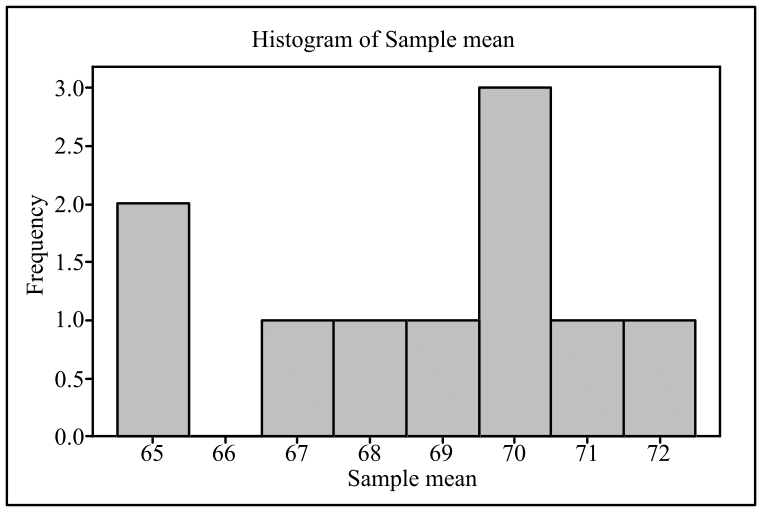
Interpretation: The obtained graph shows that maximum number of sample has mean value near 70.
To determine: Whether the population mean lies at the center of the histogram.
Solution: The population means lies at the center of the histogram.
Explanation:
The population mean is obtained as 69.4 in part (a). From the obtained histogram, it can be said that the population mean lies almost at the center of the histogram that is the center of the histogram close to the population mean.
Want to see more full solutions like this?
Chapter 18 Solutions
Statistics: Concepts and Controversies


- Name Harvard University California Institute of Technology Massachusetts Institute of Technology Stanford University Princeton University University of Cambridge University of Oxford University of California, Berkeley Imperial College London Yale University University of California, Los Angeles University of Chicago Johns Hopkins University Cornell University ETH Zurich University of Michigan University of Toronto Columbia University University of Pennsylvania Carnegie Mellon University University of Hong Kong University College London University of Washington Duke University Northwestern University University of Tokyo Georgia Institute of Technology Pohang University of Science and Technology University of California, Santa Barbara University of British Columbia University of North Carolina at Chapel Hill University of California, San Diego University of Illinois at Urbana-Champaign National University of Singapore…arrow_forwardA company found that the daily sales revenue of its flagship product follows a normal distribution with a mean of $4500 and a standard deviation of $450. The company defines a "high-sales day" that is, any day with sales exceeding $4800. please provide a step by step on how to get the answers in excel Q: What percentage of days can the company expect to have "high-sales days" or sales greater than $4800? Q: What is the sales revenue threshold for the bottom 10% of days? (please note that 10% refers to the probability/area under bell curve towards the lower tail of bell curve) Provide answers in the yellow cellsarrow_forwardFind the critical value for a left-tailed test using the F distribution with a 0.025, degrees of freedom in the numerator=12, and degrees of freedom in the denominator = 50. A portion of the table of critical values of the F-distribution is provided. Click the icon to view the partial table of critical values of the F-distribution. What is the critical value? (Round to two decimal places as needed.)arrow_forward
- A retail store manager claims that the average daily sales of the store are $1,500. You aim to test whether the actual average daily sales differ significantly from this claimed value. You can provide your answer by inserting a text box and the answer must include: Null hypothesis, Alternative hypothesis, Show answer (output table/summary table), and Conclusion based on the P value. Showing the calculation is a must. If calculation is missing,so please provide a step by step on the answers Numerical answers in the yellow cellsarrow_forwardShow all workarrow_forwardShow all workarrow_forward
 MATLAB: An Introduction with ApplicationsStatisticsISBN:9781119256830Author:Amos GilatPublisher:John Wiley & Sons Inc
 Probability and Statistics for Engineering and th...StatisticsISBN:9781305251809Author:Jay L. DevorePublisher:Cengage Learning
 Statistics for The Behavioral Sciences (MindTap C...StatisticsISBN:9781305504912Author:Frederick J Gravetter, Larry B. WallnauPublisher:Cengage Learning
 Elementary Statistics: Picturing the World (7th E...StatisticsISBN:9780134683416Author:Ron Larson, Betsy FarberPublisher:PEARSON
 The Basic Practice of StatisticsStatisticsISBN:9781319042578Author:David S. Moore, William I. Notz, Michael A. FlignerPublisher:W. H. Freeman
 Introduction to the Practice of StatisticsStatisticsISBN:9781319013387Author:David S. Moore, George P. McCabe, Bruce A. CraigPublisher:W. H. Freeman