Chapter 18, Problem 1SPPA

To determine

To show:

The graphical representation of average total cost and demand curve for automobiles.

Explanation of Solution

Average Cost function plays a pivotal role in establishing economies and diseconomies of scale.

Before the automation process and the assembly line production, cost of production of an automobile was exorbitant. This is shown in Panel a) of Figure 1. There were only few firms producing automobiles. Hence, their supply was limited. Average total cost of production curve AC shows the cost of Q1 of automobiles to be A1.

This cost reflects the average cost in 1901 when the technique of production to be used was limited and there were unspecialized workers. With assembly line production, division of labor was achieved. Automobile manufacturers were able to use specialized labor for specific activity. This greatly helped them in achieving economic of scale that reduced average cost of production.

  

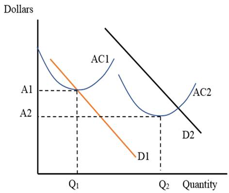
With time, there has been more use of machines that have replaced labor. This has reduced the per vehicle cost further down. This is shown by average total cost of production curve AC that shows the cost of Q2 units of automobiles to be A2 in Figure 1.

The demand curve for automobiles in 1901 was low, shown by D1 in Figure 1.People had limited financial sources to buy an automobile. Hence, they demanded fewer automobiles. With already limited supply of automobiles, the price was quite high.

By 2016, the prices have fallen because cost of production has reduced dramatically. Also, the income levels have increased for most of the consumers. This has increased their willingness to pay. Hence, the demand curve for automobiles in 2016 is higher and is shown as D2 in Figure 1.

Economics Concept Introduction

Average Total Cost:

Average total cost is expressed as the cost incurred by the firm on the production of one unit of the output, on average. It can be measured from the total cost function when the latter is divided by the number of units produced.