Chapter 18, Problem 17P

a)

Summary Introduction

To determine: System utilization rate.

Introduction: Poisson distribution is utilized to ascertain the probability of an occasion happening over a specific time period or interval. The interval can be one of time, zone, volume or separation. The probability of an event happening is discovered utilizing the equation in the Poisson distribution.

Answer to Problem 17P

The system utilization rate is 0.5500.

Explanation of Solution

Given Information:

It is given that the processing time is 4 customers per hour and there are 5 servers to process the customers.

Class	Arrivals per Hour
1	2
2	4
3	3
4	2

Calculate the system utilization:

It is calculated by adding all the total customer hours for each class and the result is divided with number of servers and customer process per hour.

$\begin{array}{c}\rho =\left[\frac{{\lambda }_1+{\lambda }_2+{\lambda }_3+{\lambda }_4}{M\mu }\right]\\ =\left[\frac{2+4+3+2}{5\times 4}\right]\\ =\left[\frac{11perhour}{20}\right]\\ =0.5500perhour\end{array}$

Here,

$\rho$ = system utilization rate

${\lambda }_1$ = total customer arrival rate for class 1

${\lambda }_2$ = total customer arrival rate for class 2

${\lambda }_3$ = total customer arrival rate for class 3

${\lambda }_4$ = total customer arrival rate for class 4

$\mu$ = customer service process rate per hour

M = number of servers

Hence the system utilization is 0.5500.

b)

Summary Introduction

To determine: The average customer waiting for service for each class and waiting in each class on average.

Answer to Problem 17P

The average wait time for service by customers for class 1 is 0.0099 hours, class 2 is 0.0142 hours, class 3 is 0.0232 hours and class 4 is 0.0361 hours. The waiting in each class on average for class 1 is 0.0199 customers, class 2 is 0.0567 customers, class 3 is 0.0696 customers and class 4 is 0.0722 customers.

Explanation of Solution

Given Information:

Class	Arrivals per Hour
1	2
2	4
3	3
4	2

It is given that the processing time is 4 customers per hour and there are 5 servers to process the customers.

Calculate the average number of customers

It is calculated by dividing the total customers arrive per hour with customer process per hour.

$\begin{array}{c}r=\left[\frac{\lambda }{\mu }\right]\\ =\left[\frac{11}{4}\right]\\ =2.75\end{array}$

Here,

r = average number of customers

$\lambda$= total customer arrival rate

$\mu$ = customer service process rate per hour

Calculate average number of customers waiting for service (L_q) using infinite-source table values for $\mu$= 2.75 and M = 5

The L_q values for $\mu$= 2.75 and M = 5 is 0.2185

Calculate A using Formula 18-16 from book:

It is calculated by subtracting 1 minus system utilization rate and multiplying the result with L_q, the whole result is divided by total customer arrival rate.

$\begin{array}{c}A=\left[\frac{{\lambda }_1+{\lambda }_2+{\lambda }_3+{\lambda }_4}{\left(1-\rho \right)L_q}\right]\\ =\left[\frac{2+4+3+2}{\left(1-0.5500\right)\times 0.2185}\right]\\ =\left[\frac{11}{0.4500\times 0.2185}\right]\\ =\left[\frac{11}{0.098325}\right]\\ =111.8739\end{array}$

Here,

L_q = average number of customers waiting for service

${\lambda }_1$ = total customer arrival rate for class 1

${\lambda }_2$ = total customer arrival rate for class 2

${\lambda }_3$ = total customer arrival rate for class 3

${\lambda }_4$ = total customer arrival rate for class 4

$\rho$ = system utilization rate

Calculate B using Formula 18-17 from book for each category:

It is calculated by multiplying number of servers with customer service process rate per hour and the result is divided by total customer arrival rate for each category.

$\begin{array}{c}{B}_0=1\\ B_1=\left[1-\left(\frac{{\lambda }_1}{M\mu }\right)\right]\\ =\left[1-\left(\frac{2}{5\times 4}\right)\right]\\ =\left[1-\left(\frac{2}{20}\right)\right]\\ =\left[1-0.1000\right]\\ =0.9000\end{array}$

$\begin{array}{c}{B}_2=\left[1-\left(\frac{{\lambda }_1+{\lambda }_2}{M\mu }\right)\right]\\ =\left[1-\left(\frac{2+4}{5\times 4}\right)\right]\\ =\left[1-\left(\frac{6}{20}\right)\right]\\ =\left[1-0.3000\right]\\ =0.7000\end{array}$

$\begin{array}{c}{B}_3=\left[1-\left(\frac{{\lambda }_1+{\lambda }_2+{\lambda }_3}{M\mu }\right)\right]\\ =\left[1-\left(\frac{2+4+3}{5\times 4}\right)\right]\\ =\left[1-\left(\frac{9}{20}\right)\right]\\ =\left[1-0.5500\right]\\ =0.4500\end{array}$

$\begin{array}{c}{B}_4=\left[1-\left(\frac{{\lambda }_1+{\lambda }_2+{\lambda }_3+{\lambda }_4}{M\mu }\right)\right]\\ =\left[1-\left(\frac{2+4+3+2}{5\times 4}\right)\right]\\ =\left[1-\left(\frac{11}{20}\right)\right]\\ =\left[1-0.4500\right]\\ =0.5500\end{array}$

Here,

${\lambda }_1$= total customer arrival rate for class 1

${\lambda }_2$= total customer arrival rate for class 2

${\lambda }_3$= total customer arrival rate for class 3

${\lambda }_4$= total customer arrival rate for class 4

$\mu$ = customer service process rate per hour

M = number of servers

$B_1$= total customer arrival rate for class 1

$B_2$= total customer arrival rate for class 2

$B_3$= total customer arrival rate for class 1

$B_4$= total customer arrival rate for class 2

Calculate the average waiting time for class 1 and class 2

It is calculated by multiplying A with B₀ and B₁, the result is divided by 1.

$\begin{array}{c}{W}_1=\left[\frac{1}{A\times B_0\times B_1}\right]\\ =\left[\frac{1}{111.8739\times 1\times 0.9000}\right]\\ =\left[\frac{1}{100.6865}\right]\\ =0.009932or0.0099hours\end{array}$

$\begin{array}{c}{W}_2=\left[\frac{1}{A\times B_1\times B_2}\right]\\ =\left[\frac{1}{111.8739\times 0.9000\times 0.7000}\right]\\ =\left[\frac{1}{70.4805}\right]\\ =0.014188or0.0142hours\end{array}$

$\begin{array}{c}{W}_3=\left[\frac{1}{A\times B_2\times B_3}\right]\\ =\left[\frac{1}{111.8739\times 0.7000\times 0.5500}\right]\\ =\left[\frac{1}{43.0714}\right]\\ =0.023217or0.0232hours\end{array}$

$\begin{array}{c}{W}_4=\left[\frac{1}{A\times B_3\times B_4}\right]\\ =\left[\frac{1}{111.8739\times 0.5500\times 0.4500}\right]\\ =\left[\frac{1}{27.6888}\right]\\ =0.036116or0.0361hours\end{array}$

Calculate the average number of customers that are waiting for service for class 1 and class 2

It is calculated by multiplying total customer arrival rate with average waiting time for units in each category.

$\begin{array}{c}{L}_1=\left[W_1\times {\lambda }_1\right]\\ =\left[0.009932\times 2\right]\\ =0.019864or0.0199customers\end{array}$

$\begin{array}{c}{L}_2=\left[W_2\times {\lambda }_2\right]\\ =\left[0.014188\times 4\right]\\ =0.056753or0.0568customers\end{array}$

$\begin{array}{c}{L}_3=\left[W_3\times {\lambda }_3\right]\\ =\left[0.023217\times 3\right]\\ =0.069652or0.0697customers\end{array}$

$\begin{array}{c}{L}_4=\left[W_4\times {\lambda }_4\right]\\ =\left[0.036116\times 2\right]\\ =0.072231or0.0722customers\end{array}$

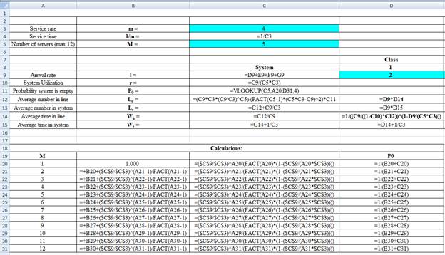
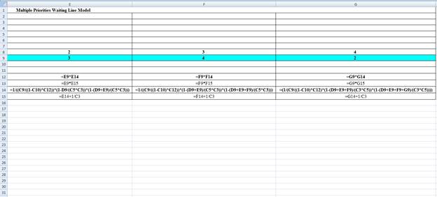
Excel Spreadsheet:

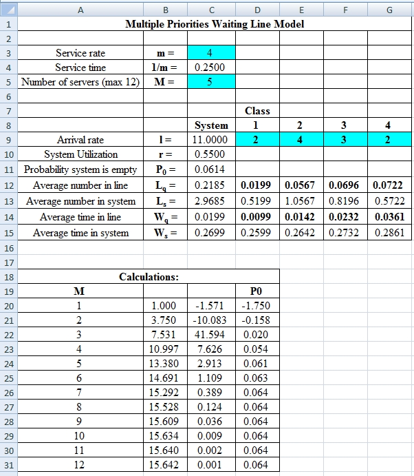
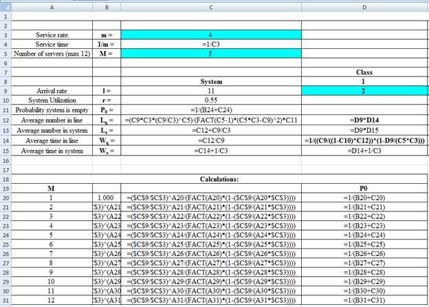
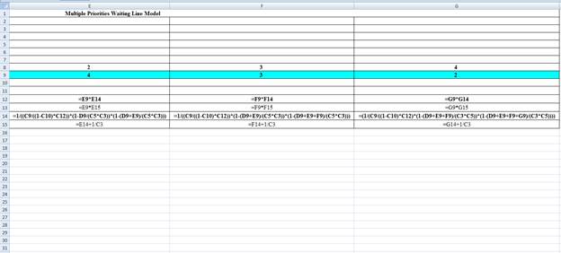
Excel Workings:

Hence the average wait time for service by customers for class 1 is 0.0099 hours, class 2 is 0.0142 hours, class 3 is 0.0232 hours and class 4 is 0.0361 hours. The waiting in each class on average for class 1 is 0.0199 customers, class 2 is 0.0567 customers, class 3 is 0.0696 customers and class 4 is 0.0722 customers.

c)

Summary Introduction

To determine: The average customer waiting for service for each class and waiting in each class on average.

Answer to Problem 17P

The average wait time for service by customers for class 1 is 0.0099 hours, class 2 is 0.0132 hours, class 3 is 0.0217 hours and class 4 is 0.0361 hours. The waiting in each class on average for class 1 is 0.0199 customers, class 2 is 0.0397 customers, class 3 is 0.0867 customers and class 4 is 0.0722 customers.

Explanation of Solution

Given Information:

It is given that the processing time is 4 customers per hour and there are 5 servers to process the customers. The second priority class is reduced to 3 units per hour by shifting some into the third party class. The arrival rate is as follows,

Class	Arrivals per Hour
1	2
2	3
3	4
4	2

Calculate the average number of customers

It is calculated by dividing the total customers arrive per hour with customer process per hour.

$\begin{array}{c}r=\left[\frac{\lambda }{\mu }\right]\\ =\left[\frac{11}{4}\right]\\ =2.75\end{array}$

Here,

r = average number of customers

$\lambda$= total customer arrival rate

$\mu$ = customer service process rate per hour

Calculate average number of customers waiting for service (L_q) using infinite-source table values for $\mu$= 2.75 and M = 5

The L_q values for $\mu$= 2.75 and M = 5 is 0.2185

Calculate A using Formula 18-16 from book

It is calculated by subtracting 1 minus system utilization rate and multiplying the result with L_q, the whole result is divided by total customer arrival rate.

$\begin{array}{c}A=\left[\frac{{\lambda }_1+{\lambda }_2+{\lambda }_3+{\lambda }_4}{\left(1-\rho \right)L_q}\right]\\ =\left[\frac{2+4+3+2}{\left(1-0.5500\right)\times 0.2185}\right]\\ =\left[\frac{11}{0.4500\times 0.2185}\right]\\ =\left[\frac{11}{0.098325}\right]\\ =111.8739\end{array}$

Here,

L_q = average number of customers waiting for service

${\lambda }_1$ = total customer arrival rate for class 1

${\lambda }_2$ = total customer arrival rate for class 2

${\lambda }_3$ = total customer arrival rate for class 3

${\lambda }_4$ = total customer arrival rate for class 4

$\rho$ = system utilization rate

Calculate B using Formula 18-17 from book for each category

It is calculated by multiplying number of servers with customer service process rate per hour and the result is divided by total customer arrival rate for each category.

$\begin{array}{c}{B}_0=1\\ B_1=\left[1-\left(\frac{{\lambda }_1}{M\mu }\right)\right]\\ =\left[1-\left(\frac{2}{5\times 4}\right)\right]\\ =\left[1-\left(\frac{2}{20}\right)\right]\\ =\left[1-0.1000\right]\\ =0.9000\end{array}$

$\begin{array}{c}{B}_2=\left[1-\left(\frac{{\lambda }_1+{\lambda }_2}{M\mu }\right)\right]\\ =\left[1-\left(\frac{2+3}{5\times 4}\right)\right]\\ =\left[1-\left(\frac{6}{20}\right)\right]\\ =\left[1-0.2500\right]\\ =0.7500\end{array}$

$\begin{array}{c}{B}_3=\left[1-\left(\frac{{\lambda }_1+{\lambda }_2+{\lambda }_3}{M\mu }\right)\right]\\ =\left[1-\left(\frac{2+3+4}{5\times 4}\right)\right]\\ =\left[1-\left(\frac{9}{20}\right)\right]\\ =\left[1-0.4500\right]\\ =0.5500\end{array}$

$\begin{array}{c}{B}_4=\left[1-\left(\frac{{\lambda }_1+{\lambda }_2+{\lambda }_3+{\lambda }_4}{M\mu }\right)\right]\\ =\left[1-\left(\frac{2+4+3+2}{5\times 4}\right)\right]\\ =\left[1-\left(\frac{11}{20}\right)\right]\\ =\left[1-0.5500\right]\\ =0.4500\end{array}$

Here,

${\lambda }_1$= total customer arrival rate for class 1

${\lambda }_2$= total customer arrival rate for class 2

${\lambda }_3$= total customer arrival rate for class 3

${\lambda }_4$= total customer arrival rate for class 4

$\mu$ = customer service process rate per hour

M = number of servers

$B_1$= total customer arrival rate for class 1

$B_2$= total customer arrival rate for class 2

$B_3$= total customer arrival rate for class 1

$B_4$= total customer arrival rate for class 2

Calculate the average waiting time for class 1 and class 2

It is calculated by multiplying A with B₀ and B₁, the result is divided by 1.

$\begin{array}{c}{W}_1=\left[\frac{1}{A\times B_0\times B_1}\right]\\ =\left[\frac{1}{111.8739\times 1\times 0.9000}\right]\\ =\left[\frac{1}{100.6865}\right]\\ =0.009932or0.0099hours\end{array}$

$\begin{array}{c}{W}_2=\left[\frac{1}{A\times B_1\times B_2}\right]\\ =\left[\frac{1}{111.8739\times 0.9000\times 0.7500}\right]\\ =\left[\frac{1}{75.5149}\right]\\ =0.013242or0.0132hours\end{array}$

$\begin{array}{c}{W}_3=\left[\frac{1}{A\times B_2\times B_3}\right]\\ =\left[\frac{1}{111.8739\times 0.7500\times 0.5500}\right]\\ =\left[\frac{1}{46.1480}\right]\\ =0.021669or0.0217hours\end{array}$

$\begin{array}{c}{W}_4=\left[\frac{1}{A\times B_3\times B_4}\right]\\ =\left[\frac{1}{111.8739\times 0.5500\times 0.4500}\right]\\ =\left[\frac{1}{27.6888}\right]\\ =0.036116or0.0361hours\end{array}$

Calculate the average number of customers that are waiting for service for class 1 and class 2

It is calculated by multiplying total customer arrival rate with average waiting time for units in each category.

$\begin{array}{c}{L}_1=\left[W_1\times {\lambda }_1\right]\\ =\left[0.009932\times 2\right]\\ =0.019864or0.0199customers\end{array}$

$\begin{array}{c}{L}_2=\left[W_2\times {\lambda }_2\right]\\ =\left[0.013242\times 3\right]\\ =0.039727or0.0397customers\end{array}$

$\begin{array}{c}{L}_3=\left[W_3\times {\lambda }_3\right]\\ =\left[0.021669\times 4\right]\\ =0.086678or0.0867customers\end{array}$

$\begin{array}{c}{L}_4=\left[W_4\times {\lambda }_4\right]\\ =\left[0.036116\times 2\right]\\ =0.072231or0.0722customers\end{array}$

Excel Spreadsheet:

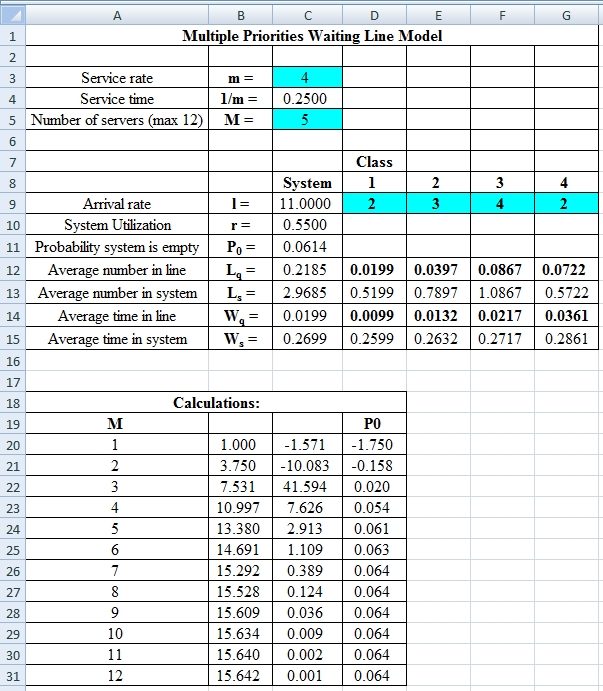
Excel Workings:

Hence the average wait time for service by customers for class 1 is 0.0099 hours, class 2 is 0.0132 hours, class 3 is 0.0217 hours and class 4 is 0.0361 hours. The waiting in each class on average for class 1 is 0.0199 customers, class 2 is 0.0397 customers, class 3 is 0.0867 customers and class 4 is 0.0722 customers.

d)

Summary Introduction

To determine: The observations based on the results from part c.

Answer to Problem 17P

Changing several arrivals from Class 2 to Class 3 decreased the average wait time. Additionally, the average number waiting reduced for Class 2, while the average number waiting for Class 3 increased by the same amount.

Explanation of Solution

Calculate the change in average wait time for each class.

It is calculated by subtracting the final answer for average wait time for service by customers from part b with the final answer for average wait time for service by customers from part c.

$\begin{array}{c}ChangeinAverageTim{e}_{Class1}=\left[0.0099-0.0099\right]\\ =0hours\end{array}$

$\begin{array}{c}ChangeinAverageTim{e}_{Class2}=\left[0.0142-0.0132\right]\\ =0.0010hours\end{array}$

$\begin{array}{c}ChangeinAverageTim{e}_{Class3}=\left[0.0232-0.0217\right]\\ =0.0015hours\end{array}$

$\begin{array}{c}ChangeinAverageTim{e}_{Class3}=\left[0.0361-0.0361\right]\\ =0hours\end{array}$

The above results suggest that there is a decrease in average wait time for class 2 and class 3. Class 1 and 4 remains constant.

Calculate the change in average number waiting for each class.

It is calculated by subtracting the final answer for waiting on average from part b with the final answer for waiting on average from part c.

$\begin{array}{c}ChangeinAverageWaitin{g}_{Class1}=\left[0.0099-0.0099\right]\\ =0customers\end{array}$

$\begin{array}{c}ChangeinAverageTim{e}_{Class2}=\left[0.0567-0.0397\right]\\ =0.0170customers\end{array}$

$\begin{array}{c}ChangeinAverageTim{e}_{Class3}=\left[0.0867-0.0696\right]\\ =0.0171customers\end{array}$

$\begin{array}{c}ChangeinAverageTim{e}_{Class4}=\left[0.0722-0.0722\right]\\ =0customers\end{array}$

The above results suggest that there is a decrease in average waiting for class 2 and an increase in class 3. Class 1 and 4 remains constant.