
Videos
(a)
To test: Whether there is any statistically significant evidence at the
α=0.10 level against the hypothesis that the
(a)
Answer to Problem 17.38E
There is statistically significant difference at α=0.10 level against the hypothesis that the mean is 32,500 pounds.
Explanation of Solution
Given info:
The data represents the sample of strength of pieces of wood and standard deviation 3,000 pounds.
Calculation:
STATE:
The strength of pieces of wood follows
PLAN:
Parameter:
Define the parameter μ as the mean strength of pieces of wood.
The hypotheses are given below:
The claim of the problem is the mean strength is different from 32,500.
Null Hypothesis:
H0:μ=32,500
That is, the mean strength is equal to 32,500.
Alternative hypothesis:
Ha:μ≠32,500
That is, the mean strength is not equal to 32,500.
SOLVE:
Conditions for valid test:
A sample of 20 pieces of wood is randomly selected and strength of pieces of wood follows normal distribution with standard deviation σ=3,000.
Test statistic and P-value:
Software procedure:
Step-by-step procedure to obtain test statistic and P-value using the MINITAB software:
- Choose Stat > Basic Statistics > 1-Sample Z.
- In Samples in Column, enter the column of Strength of pieces.
- In Standard deviation, enter 3,000.
- In Perform hypothesis test, enter the test mean as 32,500.
- Check Options, enter Confidence level as 90.
- Choose not equal in alternative.
- Click OK in all dialogue boxes.
Output using the MINITAB software is given below:
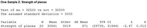
From the MINITAB output, the test statistic is –2.47 and the P-value is 0.013.
Decision criteria for the P-value method:
If P-value≤α(=0.10), then reject the null hypothesis (H0).
If P-value>α(=0.10), then fail to reject the null hypothesis (H0).
CONCLUDE:
Use a significance level, α=0.10.
Here, P-value is 0.013, which is lesser than the value of α=0.10.
That is, P-value(=0.013)<α(=0.10).
Therefore, the null hypothesis is rejected.
Thus, there is statistically significant at α=0.10 level against the hypothesis that the mean is 32,500 pounds.
(b)
To test: Whether there is any statistically significant evidence at the α=0.10 level against the hypothesis that the mean is 31,500 pounds or not for the two-sided alternative.
(b)
Answer to Problem 17.38E
There is no statistically significant difference at α=0.10 level against the hypothesis that the mean is 31,500 pounds.
Explanation of Solution
Calculation:
STATE:
Is there statistically significant evidence at the α=0.10 level against the hypothesis that the mean is 31,500 pounds for the two-sided alternative?
PLAN:
Parameter:
Define the parameter μ as the mean strength of pieces of wood.
The hypotheses are given below:
The claim of the problem is the mean strength is different from 31,500.
Null Hypothesis:
H0:μ=31,500
That is, the mean strength is equal to 31,500.
Alternative hypothesis:
Ha:μ≠31,500
That is, the mean strength is not equal to 31,500.
SOLVE:
Conditions for valid test:
A sample of 20 pieces of wood is randomly selected and strength of pieces of wood follows normal distribution with standard deviation σ=3,000.
Test statistic and P-value:
Software procedure:
Step-by-step procedure to obtain test statistic and P-value using the MINITAB software:
- Choose Stat > Basic Statistics > 1-Sample Z.
- In Samples in Column, enter the column of Strength of pieces.
- In Standard deviation, enter 3,000.
- In Perform hypothesis test, enter the test mean as 31,500.
- Check Options, enter Confidence level as 90.
- Choose not equal in alternative.
- Click OK in all dialogue boxes.
Output using the MINITAB software is given below:
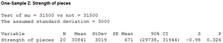
From the MINITAB output, the test statistic is –0.98 and the P-value is 0.326.
CONCLUDE:
Use a significance level, α=0.10.
Here, P-value is 0.326, which is greater than the value of α=0.10.
That is, P-value(=0.326)>α(=0.10).
Therefore, the null hypothesis is not rejected.
Thus, there is no statistically significant difference at α=0.10 level against the hypothesis that the mean is 31,500 pounds.
Want to see more full solutions like this?
Chapter 17 Solutions
BASIC PRACTICE OF STATISTICS+LAUNCHPAD


- If, based on a sample size of 900,a political candidate finds that 509people would vote for him in a two-person race, what is the 95%confidence interval for his expected proportion of the vote? Would he be confident of winning based on this poll? Question content area bottom Part 1 A 9595% confidence interval for his expected proportion of the vote is (Use ascending order. Round to four decimal places as needed.)arrow_forwardQuestions An insurance company's cumulative incurred claims for the last 5 accident years are given in the following table: Development Year Accident Year 0 2018 1 2 3 4 245 267 274 289 292 2019 255 276 288 294 2020 265 283 292 2021 263 278 2022 271 It can be assumed that claims are fully run off after 4 years. The premiums received for each year are: Accident Year Premium 2018 306 2019 312 2020 318 2021 326 2022 330 You do not need to make any allowance for inflation. 1. (a) Calculate the reserve at the end of 2022 using the basic chain ladder method. (b) Calculate the reserve at the end of 2022 using the Bornhuetter-Ferguson method. 2. Comment on the differences in the reserves produced by the methods in Part 1.arrow_forwardA population that is uniformly distributed between a=0and b=10 is given in sample sizes 50( ), 100( ), 250( ), and 500( ). Find the sample mean and the sample standard deviations for the given data. Compare your results to the average of means for a sample of size 10, and use the empirical rules to analyze the sampling error. For each sample, also find the standard error of the mean using formula given below. Standard Error of the Mean =sigma/Root Complete the following table with the results from the sampling experiment. (Round to four decimal places as needed.) Sample Size Average of 8 Sample Means Standard Deviation of 8 Sample Means Standard Error 50 100 250 500arrow_forward
- A survey of 250250 young professionals found that two dash thirdstwo-thirds of them use their cell phones primarily for e-mail. Can you conclude statistically that the population proportion who use cell phones primarily for e-mail is less than 0.720.72? Use a 95% confidence interval. Question content area bottom Part 1 The 95% confidence interval is left bracket nothing comma nothing right bracket0.60820.6082, 0.72510.7251. As 0.720.72 is within the limits of the confidence interval, we cannot conclude that the population proportion is less than 0.720.72. (Use ascending order. Round to four decimal places as needed.)arrow_forwardI need help with this problem and an explanation of the solution for the image described below. (Statistics: Engineering Probabilities)arrow_forwardA survey of 250 young professionals found that two-thirds of them use their cell phones primarily for e-mail. Can you conclude statistically that the population proportion who use cell phones primarily for e-mail is less than 0.72? Use a 95% confidence interval. Question content area bottom Part 1 The 95% confidence interval is [ ], [ ] As 0.72 is ▼ above the upper limit within the limits below the lower limit of the confidence interval, we ▼ can cannot conclude that the population proportion is less than 0.72. (Use ascending order. Round to four decimal places as needed.)arrow_forward
- I need help with this problem and an explanation of the solution for the image described below. (Statistics: Engineering Probabilities)arrow_forwardI need help with this problem and an explanation of the solution for the image described below. (Statistics: Engineering Probabilities)arrow_forwardI need help with this problem and an explanation of the solution for the image described below. (Statistics: Engineering Probabilities)arrow_forward
- Questions An insurance company's cumulative incurred claims for the last 5 accident years are given in the following table: Development Year Accident Year 0 2018 1 2 3 4 245 267 274 289 292 2019 255 276 288 294 2020 265 283 292 2021 263 278 2022 271 It can be assumed that claims are fully run off after 4 years. The premiums received for each year are: Accident Year Premium 2018 306 2019 312 2020 318 2021 326 2022 330 You do not need to make any allowance for inflation. 1. (a) Calculate the reserve at the end of 2022 using the basic chain ladder method. (b) Calculate the reserve at the end of 2022 using the Bornhuetter-Ferguson method. 2. Comment on the differences in the reserves produced by the methods in Part 1.arrow_forwardQuestions An insurance company's cumulative incurred claims for the last 5 accident years are given in the following table: Development Year Accident Year 0 2018 1 2 3 4 245 267 274 289 292 2019 255 276 288 294 2020 265 283 292 2021 263 278 2022 271 It can be assumed that claims are fully run off after 4 years. The premiums received for each year are: Accident Year Premium 2018 306 2019 312 2020 318 2021 326 2022 330 You do not need to make any allowance for inflation. 1. (a) Calculate the reserve at the end of 2022 using the basic chain ladder method. (b) Calculate the reserve at the end of 2022 using the Bornhuetter-Ferguson method. 2. Comment on the differences in the reserves produced by the methods in Part 1.arrow_forwardFrom a sample of 26 graduate students, the mean number of months of work experience prior to entering an MBA program was 34.67. The national standard deviation is known to be18 months. What is a 90% confidence interval for the population mean? Question content area bottom Part 1 A 9090% confidence interval for the population mean is left bracket nothing comma nothing right bracketenter your response here,enter your response here. (Use ascending order. Round to two decimal places as needed.)arrow_forward
 MATLAB: An Introduction with ApplicationsStatisticsISBN:9781119256830Author:Amos GilatPublisher:John Wiley & Sons Inc
 Probability and Statistics for Engineering and th...StatisticsISBN:9781305251809Author:Jay L. DevorePublisher:Cengage Learning
 Statistics for The Behavioral Sciences (MindTap C...StatisticsISBN:9781305504912Author:Frederick J Gravetter, Larry B. WallnauPublisher:Cengage Learning
 Elementary Statistics: Picturing the World (7th E...StatisticsISBN:9780134683416Author:Ron Larson, Betsy FarberPublisher:PEARSON
 The Basic Practice of StatisticsStatisticsISBN:9781319042578Author:David S. Moore, William I. Notz, Michael A. FlignerPublisher:W. H. Freeman
 Introduction to the Practice of StatisticsStatisticsISBN:9781319013387Author:David S. Moore, George P. McCabe, Bruce A. CraigPublisher:W. H. Freeman