Concept explainers
Videos
A sample containing years to maturity and yield (%) for 40 corporate bonds is contained in the data file named CorporateBonds (Barron’s, April 2, 2012).
- a. Develop a
scatter diagram of the data using x = years to maturity as the independent variable. Does a simple linear regression model appear to be appropriate? - b. Develop an estimated regression equation with x = years to maturity and x2 as the independent variables.
- c. As an alternative to fitting a second-order model, fit a model using the natural logarithm of price as the independent variable; that is, ŷ = b0 + b1ln(x). Does the estimated regression using the natural logarithm of x provide a better fit than the estimated regression developed in part (b)? Explain.
a.
Construct a scatter diagram of the data using
Decide whether a simple linear regression model appears to be appropriate.
Answer to Problem 29SE
The scatter diagram of the data using
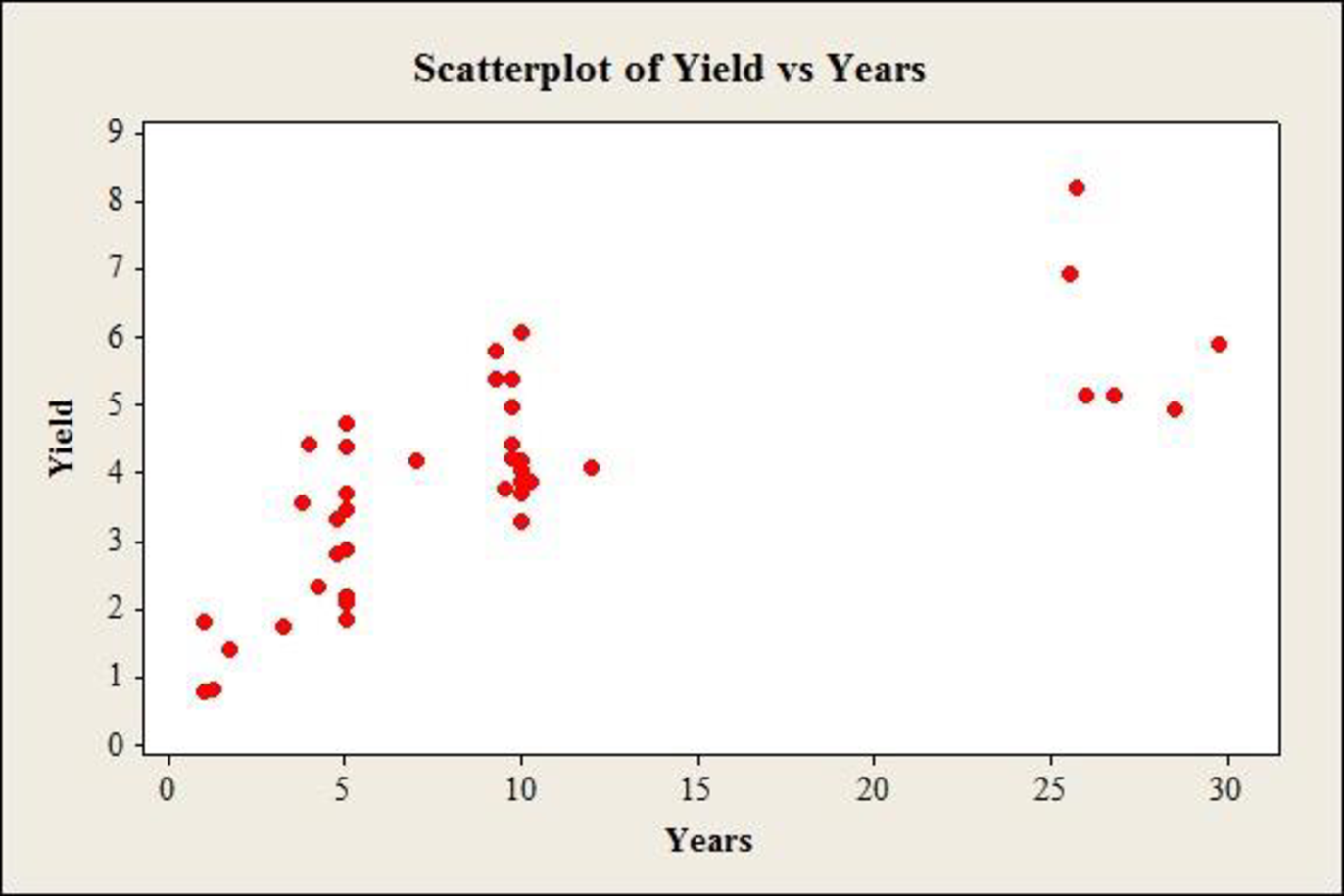
A simple linear regression model does not appear to be appropriate.
Explanation of Solution
Calculation:
The data gives information on yield (%) of 40 corporate bonds and the respective years to maturity.
Scatterplot:
Software procedure:
Step by step procedure to draw scatter diagram using MINITAB software is given below:
- Choose Graph > Scatterplot.
- Choose Simple, and then click OK.
- In Y–variables, enter the column of Yield.
- In X–variables enter the column of Years.
- Click OK.
Observation:
The scatterplot shows a gradual increase in the yield, at a decreasing rate, with increase in years up to 25. After this, there is a reduction in the values of yield. Thus, a simple linear regression model does not appear to be appropriate.
b.
Develop an estimated multiple regression equation with
Answer to Problem 29SE
The estimated multiple regression equation with
Explanation of Solution
Calculation:
Square transformation:
Software procedure:
Step by step procedure to make square transformation using MINITAB software is given as,
- Choose Calc > Calculator.
- In Store result in variable, enter YearsSq.
- In Expression, enter ‘Years’^2.
- Click OK.
The squared variable is stored in the column of ‘YearsSq’.
Regression:
Software procedure:
Step by step procedure to obtain the regression equation using MINITAB software:
- Choose Stat > Regression > General Regression.
- Under Responses, enter the column of Yield.
- Under Model, enter the columns of Years, YearsSq.
- Click OK.
Output using MINITAB software is given below:
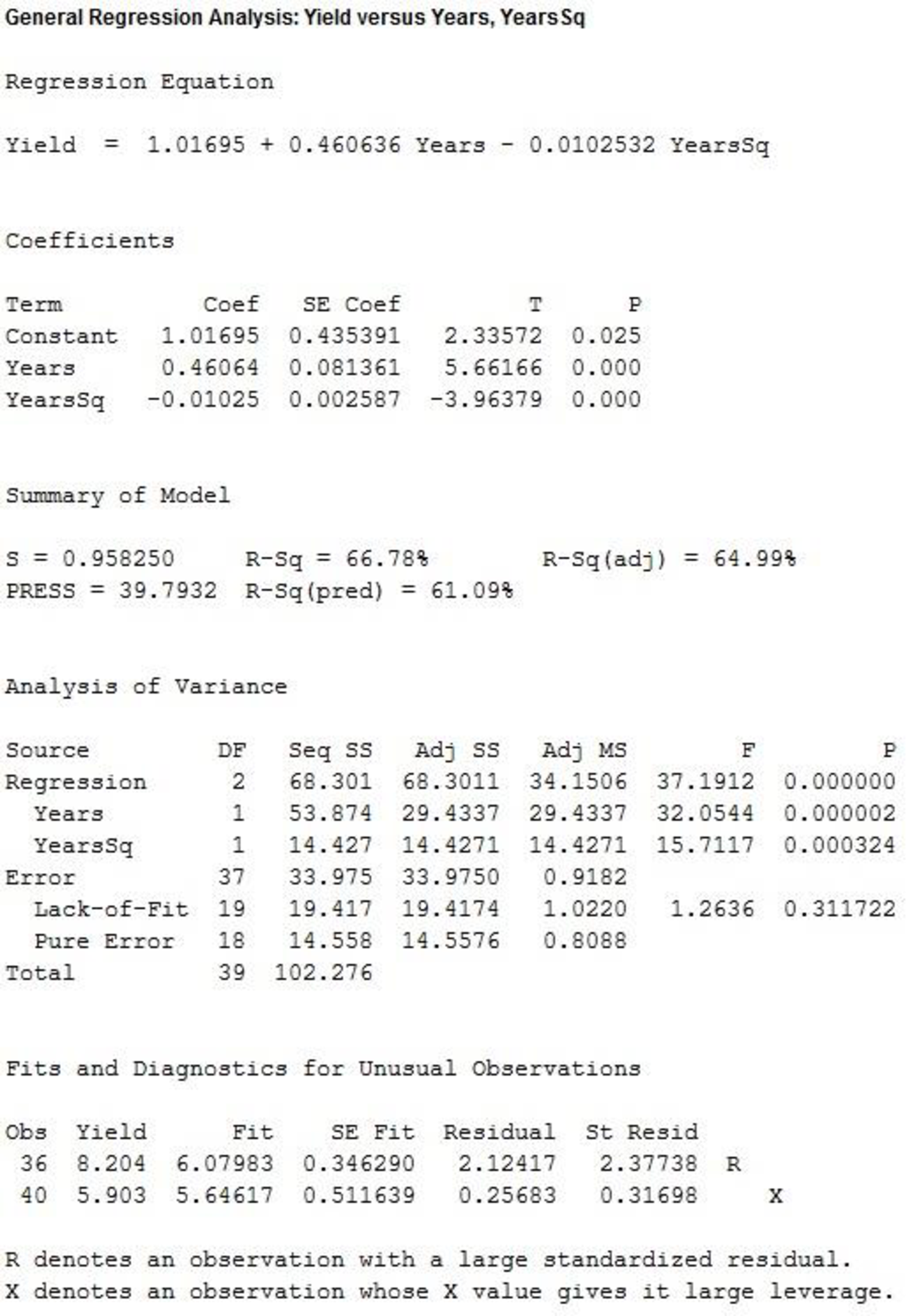
From the output, the estimated multiple regression equation with
c.
Develop an estimated multiple regression equation using the natural logarithm of years as the independent variable.
Explain whether the current regression provides a better fit than the estimated regression developed in part b.
Answer to Problem 29SE
The estimated multiple regression equation using the natural logarithm of years as the independent variable is:
The estimated regression using the natural logarithm of x provides a better fit than the estimated regression developed in part b.
Explanation of Solution
Calculation:
Logarithmic transformation:
Software procedure:
Step by step procedure to make logarithmic transformation using MINITAB software is given as,
- Choose Calc > Calculator.
- In Store result in variable, enter Years.
- In Expression, enter ln(‘Years’).
- Click OK.
The logarithm of the variable is stored in the column of ‘ln(‘Years’)’.
Regression:
Software procedure:
Step by step procedure to obtain the regression equation using MINITAB software:
- Choose Stat > Regression > General Regression.
- Under Responses, enter the column of Yield.
- Under Model, enter the columns of ln(Years).
- Click OK.
Output using MINITAB software is given below:
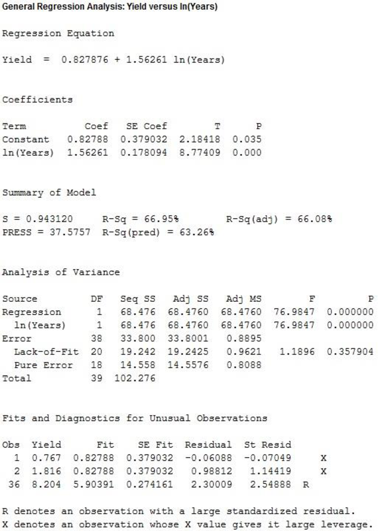
From the output, the estimated multiple regression equation using the natural logarithm of years as the independent variable is:
Adjusted-
The adjusted
The value of adjusted
The value of adjusted
Evidently, the current regression equation effectively explains more of the variation the response variable, than the second regression equation.
Thus, the estimated regression using the natural logarithm of x provides a better fit than the estimated regression developed in part b.
Want to see more full solutions like this?
Chapter 16 Solutions
STATISTICS F/BUSINESS+ECONOMICS-TEXT


- ons 12. A sociologist hypothesizes that the crime rate is higher in areas with higher poverty rate and lower median income. She col- lects data on the crime rate (crimes per 100,000 residents), the poverty rate (in %), and the median income (in $1,000s) from 41 New England cities. A portion of the regression results is shown in the following table. Standard Coefficients error t stat p-value Intercept -301.62 549.71 -0.55 0.5864 Poverty 53.16 14.22 3.74 0.0006 Income 4.95 8.26 0.60 0.5526 a. b. Are the signs as expected on the slope coefficients? Predict the crime rate in an area with a poverty rate of 20% and a median income of $50,000. 3. Using data from 50 workarrow_forward2. The owner of several used-car dealerships believes that the selling price of a used car can best be predicted using the car's age. He uses data on the recent selling price (in $) and age of 20 used sedans to estimate Price = Po + B₁Age + ε. A portion of the regression results is shown in the accompanying table. Standard Coefficients Intercept 21187.94 Error 733.42 t Stat p-value 28.89 1.56E-16 Age -1208.25 128.95 -9.37 2.41E-08 a. What is the estimate for B₁? Interpret this value. b. What is the sample regression equation? C. Predict the selling price of a 5-year-old sedan.arrow_forwardian income of $50,000. erty rate of 13. Using data from 50 workers, a researcher estimates Wage = Bo+B,Education + B₂Experience + B3Age+e, where Wage is the hourly wage rate and Education, Experience, and Age are the years of higher education, the years of experience, and the age of the worker, respectively. A portion of the regression results is shown in the following table. ni ogolloo bash 1 Standard Coefficients error t stat p-value Intercept 7.87 4.09 1.93 0.0603 Education 1.44 0.34 4.24 0.0001 Experience 0.45 0.14 3.16 0.0028 Age -0.01 0.08 -0.14 0.8920 a. Interpret the estimated coefficients for Education and Experience. b. Predict the hourly wage rate for a 30-year-old worker with four years of higher education and three years of experience.arrow_forward
- 1. If a firm spends more on advertising, is it likely to increase sales? Data on annual sales (in $100,000s) and advertising expenditures (in $10,000s) were collected for 20 firms in order to estimate the model Sales = Po + B₁Advertising + ε. A portion of the regression results is shown in the accompanying table. Intercept Advertising Standard Coefficients Error t Stat p-value -7.42 1.46 -5.09 7.66E-05 0.42 0.05 8.70 7.26E-08 a. Interpret the estimated slope coefficient. b. What is the sample regression equation? C. Predict the sales for a firm that spends $500,000 annually on advertising.arrow_forwardCan you help me solve problem 38 with steps im stuck.arrow_forwardHow do the samples hold up to the efficiency test? What percentages of the samples pass or fail the test? What would be the likelihood of having the following specific number of efficiency test failures in the next 300 processors tested? 1 failures, 5 failures, 10 failures and 20 failures.arrow_forward
- The battery temperatures are a major concern for us. Can you analyze and describe the sample data? What are the average and median temperatures? How much variability is there in the temperatures? Is there anything that stands out? Our engineers’ assumption is that the temperature data is normally distributed. If that is the case, what would be the likelihood that the Safety Zone temperature will exceed 5.15 degrees? What is the probability that the Safety Zone temperature will be less than 4.65 degrees? What is the actual percentage of samples that exceed 5.25 degrees or are less than 4.75 degrees? Is the manufacturing process producing units with stable Safety Zone temperatures? Can you check if there are any apparent changes in the temperature pattern? Are there any outliers? A closer look at the Z-scores should help you in this regard.arrow_forwardNeed help pleasearrow_forwardPlease conduct a step by step of these statistical tests on separate sheets of Microsoft Excel. If the calculations in Microsoft Excel are incorrect, the null and alternative hypotheses, as well as the conclusions drawn from them, will be meaningless and will not receive any points. 4. One-Way ANOVA: Analyze the customer satisfaction scores across four different product categories to determine if there is a significant difference in means. (Hints: The null can be about maintaining status-quo or no difference among groups) H0 = H1=arrow_forward
- Please conduct a step by step of these statistical tests on separate sheets of Microsoft Excel. If the calculations in Microsoft Excel are incorrect, the null and alternative hypotheses, as well as the conclusions drawn from them, will be meaningless and will not receive any points 2. Two-Sample T-Test: Compare the average sales revenue of two different regions to determine if there is a significant difference. (Hints: The null can be about maintaining status-quo or no difference among groups; if alternative hypothesis is non-directional use the two-tailed p-value from excel file to make a decision about rejecting or not rejecting null) H0 = H1=arrow_forwardPlease conduct a step by step of these statistical tests on separate sheets of Microsoft Excel. If the calculations in Microsoft Excel are incorrect, the null and alternative hypotheses, as well as the conclusions drawn from them, will be meaningless and will not receive any points 3. Paired T-Test: A company implemented a training program to improve employee performance. To evaluate the effectiveness of the program, the company recorded the test scores of 25 employees before and after the training. Determine if the training program is effective in terms of scores of participants before and after the training. (Hints: The null can be about maintaining status-quo or no difference among groups; if alternative hypothesis is non-directional, use the two-tailed p-value from excel file to make a decision about rejecting or not rejecting the null) H0 = H1= Conclusion:arrow_forwardPlease conduct a step by step of these statistical tests on separate sheets of Microsoft Excel. If the calculations in Microsoft Excel are incorrect, the null and alternative hypotheses, as well as the conclusions drawn from them, will be meaningless and will not receive any points. The data for the following questions is provided in Microsoft Excel file on 4 separate sheets. Please conduct these statistical tests on separate sheets of Microsoft Excel. If the calculations in Microsoft Excel are incorrect, the null and alternative hypotheses, as well as the conclusions drawn from them, will be meaningless and will not receive any points. 1. One Sample T-Test: Determine whether the average satisfaction rating of customers for a product is significantly different from a hypothetical mean of 75. (Hints: The null can be about maintaining status-quo or no difference; If your alternative hypothesis is non-directional (e.g., μ≠75), you should use the two-tailed p-value from excel file to…arrow_forward
 Functions and Change: A Modeling Approach to Coll...AlgebraISBN:9781337111348Author:Bruce Crauder, Benny Evans, Alan NoellPublisher:Cengage Learning
 Glencoe Algebra 1, Student Edition, 9780079039897...AlgebraISBN:9780079039897Author:CarterPublisher:McGraw Hill
 Big Ideas Math A Bridge To Success Algebra 1: Stu...AlgebraISBN:9781680331141Author:HOUGHTON MIFFLIN HARCOURTPublisher:Houghton Mifflin Harcourt
 College AlgebraAlgebraISBN:9781305115545Author:James Stewart, Lothar Redlin, Saleem WatsonPublisher:Cengage Learning
 Algebra and Trigonometry (MindTap Course List)AlgebraISBN:9781305071742Author:James Stewart, Lothar Redlin, Saleem WatsonPublisher:Cengage Learning