Concept explainers
Videos
1.
Complete the F table.
Make a decision to retain or reject the null hypothesis that the multiple regression equation can be used to significantly predict health.
1.
Answer to Problem 28CAP
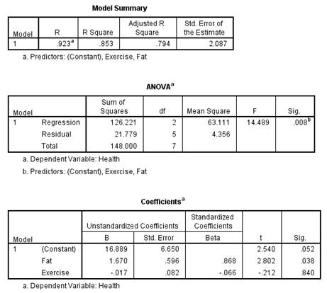
The completed F table is,
| Source of variation | SS | df | MS | |
| Regression | 126.22 | 2 | 63.11 | 14.48 |
| Residual (error) | 21.78 | 5 | 4.36 | |
| Total | 148.00 | 7 |
The decision is to reject the null hypothesis.
Theregression equation significantly predicts variance in criterion variable (Y) health [BMI].
Explanation of Solution
Calculation:
The given information is that, the researcher has tested whether ‘daily intake of fat (in grams)’ and ‘amount of exercise (in minutes)’ can predict health (measured using a body mass index [BMI] scale.
The formula for test statistic is,
Decision rules:
- If the test statistic value is greater than the critical value, then reject the null hypothesis
- If the test statistic value is smaller than the critical value, then retain the null hypothesis
Null hypothesis:
Alternative hypothesis:
Software procedure:
Step by step procedure to obtain test statistic value using SPSS software is given as,
- Choose Variable view.
- Under the name, enter the name as Fat, Exercise, Health.
- Choose Data view, enter the data.
- Choose Analyze>Regression>Linear.
- In Dependents, enter the column of Health.
- In Independents, enter the column of Fat, and Exercise.
- Click OK.
Output using SPSS software is given below:
The table of F is,
| Source of variation | SS | df | MS | |
| Regression | 126.22 | 2 | 63.11 | 14.48 |
| Residual (error) | 21.78 | 5 | 4.36 | |
| Total | 148.00 | 7 |
Table 1
Critical value:
The considered significance level is
The degrees of freedom for regression are 2, the degrees of freedom for residual are 5.
From the Appendix C: Table C.3-Critical values for F distribution:
- Locate the value 2 in degrees of freedomnumerator row.
- Locate the value 5 in degrees of freedomdenominator row.
- Locate the 0.05 level of significance (value in lightface type) in combined row.
- The intersecting value that corresponds to the (2, 5) with level of significance 0.05 is 5.79.
Thus, the critical value for
Conclusion:
The value of test statistic is 14.48.
The critical value is 5.79.
The test statistic value is greater than the critical value.
The test statistic value falls under critical region.
Hence the null hypothesis is rejected.
Thus, the regression equation significantly predicts variance in criterion variable (Y) health [BMI].
2.
Determine which predictor variable or variables, when added to the multiple regression equation, significantly contributed to predictions in Y (health).
2.
Answer to Problem 28CAP
The predictor variabledaily intake of fat significantly contributed to predictions in Y (health) when added to the multiple regression equation.
Explanation of Solution
Calculation:
The given information is that, a sample of 8 scores is recorded. The predictor variables are ‘daily intake of fat (in grams)
Relative contribution to fat
Null hypothesis:
Alternative hypothesis:
The predictor variable fat is tested. The other predictor variable that is not tested is ‘Exercise’. Calculate the correlation between ‘Exercise’ and ‘Health[BMI]’.
Software procedure:
Step by step procedure to obtain correlation using SPSS software is given as,
- Choose Variable view.
- Under the name, enter the name as Health, Exercise.
- Choose Data view, enter the data.
- Choose Analyze>Correlate>Bivariate.
- In variables, enter the Health, and Exercise.
- Click OK.
Output using SPSS software is given below:
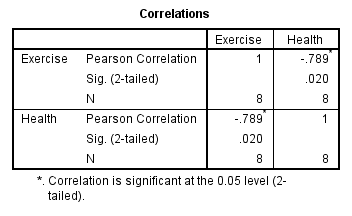
The correlation between ‘Exercise’ and ‘Health [BMI]’ is –0.789.
The value of
The formula for
The calculation of sums of squares is,
|
Health [BMI] (Y) | |
| 32 | 1,024 |
| 34 | 1,156 |
| 23 | 529 |
| 33 | 1,089 |
| 28 | 784 |
| 27 | 729 |
| 25 | 625 |
| 22 | 484 |
Table 2
Substitute,
The contribution of
From the F table, the value of
The contribution of
Reproduce the F table by replacing,
Since there would be only one predictor variable, the degrees of freedom for regression would be 1.
The mean sums of squares for regression is,
The F statistic value is,
The change F table with
| Source of variation | SS | df | MS | |
| Regression | 34.09 | 1 | 34.09 | 7.82 |
| Residual (error) | 21.78 | 5 | 4.36 | |
| Total | 148.00 | 7 |
Critical value:
The considered significance level is
The degrees of freedom for regression are 1, the degrees of freedom for residual are 5.
From the Appendix C: Table C.3-Critical values for F distribution:
- Locate the value 1 in degrees of freedom numerator row.
- Locate the value 5 in degrees of freedom denominator row.
- Locate the 0.05 level of significance (value in lightface type) in combined row.
- The intersecting value that corresponds to the (1, 5) with level of significance 0.05 is 6.61.
Thus, the critical value for
Conclusion:
The value of test statistic is 7.82.
The critical value is 6.61.
The test statistic value is greater than the critical value.
The test statistic value falls under critical region.
Hence the null hypothesis is rejected.
Thus, adding fat
Relative contribution to exercise
Null hypothesis:
Alternative hypothesis:
The predictor variable exercise is tested. The other predictor variable that is not tested is ‘fat’. Calculate the correlation between ‘fat’ and ‘Health [BMI]’.
Software procedure:
Step by step procedure to obtain correlation using SPSS software is given as,
- Choose Variable view.
- Under the name, enter the name as Health, Fat.
- Choose Data view, enter the data.
- Choose Analyze>Correlate>Bivariate.
- In variables, enter the Health, and Fat.
- Click OK.
Output using SPSS software is given below:
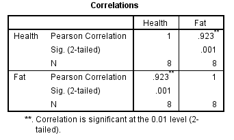
The correlation between ‘fat’ and ‘Health [BMI]’ is 0.923.
The value of
The value for
From the F table, the value of
The contribution of
Reproduce the F table by replacing,
Since there would be only one predictor variable, the degrees of freedom for regression would be 1.
The mean sums of squares for regression is,
The F statistic value is,
The change F table with
| Source of variation | SS | df | MS | |
| Regression | 0.14 | 1 | 0.14 | 0.03 |
| Residual (error) | 21.78 | 5 | 4.36 | |
| Total | 148.00 | 7 |
The critical value for F table with
Conclusion:
The value of test statistic is 0.03.
The critical value is 6.61.
The test statistic value is less than the critical value.
The test statistic value does not fall under critical region.
Hence the null hypothesis is retained.
Thus, adding exercise
Hence, the predictor variable daily intake of fat significantly contributed to predictions in Y (health) when added to the multiple regression equation.
Want to see more full solutions like this?
Chapter 16 Solutions
Statistics for the Behavioral Sciences


- Definition of null hypothesis from the textbook Definition of alternative hypothesis from the textbook Imagine this: you suspect your beloved Chicken McNugget is shrinking. Inflation is hitting everything else, so why not the humble nugget too, right? But your sibling thinks you’re just being dramatic—maybe you’re just extra hungry today. Determined to prove them wrong, you take matters (and nuggets) into your own hands. You march into McDonald’s, get two 20-piece boxes, and head home like a scientist on a mission. Now, before you start weighing each nugget like they’re precious gold nuggets, let’s talk hypotheses. The average weight of nuggets as mentioned on the box is 16 g each. Develop your null and alternative hypotheses separately. Next, you weigh each nugget with the precision of a jeweler and find they average out to 15.5 grams. You also conduct a statistical analysis, and the p-value turns out to be 0.01. Based on this information, answer the following questions. (Remember,…arrow_forwardBusiness Discussarrow_forwardCape Fear Community Colle X ALEKS ALEKS - Dorothy Smith - Sec X www-awu.aleks.com/alekscgi/x/Isl.exe/10_u-IgNslkr7j8P3jH-IQ1w4xc5zw7yX8A9Q43nt5P1XWJWARE... Section 7.1,7.2,7.3 HW 三 Question 21 of 28 (1 point) | Question Attempt: 5 of Unlimited The proportion of phones that have more than 47 apps is 0.8783 Part: 1 / 2 Part 2 of 2 (b) Find the 70th The 70th percentile of the number of apps. Round the answer to two decimal places. percentile of the number of apps is Try again Skip Part Recheck Save 2025 Mcarrow_forward
- Hi, I need to sort out where I went wrong. So, please us the data attached and run four separate regressions, each using the Recruiters rating as the dependent variable and GMAT, Accept Rate, Salary, and Enrollment, respectively, as a single independent variable. Interpret this equation. Round your answers to four decimal places, if necessary. If your answer is negative number, enter "minus" sign. Equation for GMAT: Ŷ = _______ + _______ GMAT Equation for Accept Rate: Ŷ = _______ + _______ Accept Rate Equation for Salary: Ŷ = _______ + _______ Salary Equation for Enrollment: Ŷ = _______ + _______ Enrollmentarrow_forwardQuestion 21 of 28 (1 point) | Question Attempt: 5 of Unlimited Dorothy ✔ ✓ 12 ✓ 13 ✓ 14 ✓ 15 ✓ 16 ✓ 17 ✓ 18 ✓ 19 ✓ 20 = 21 22 > How many apps? According to a website, the mean number of apps on a smartphone in the United States is 82. Assume the number of apps is normally distributed with mean 82 and standard deviation 30. Part 1 of 2 (a) What proportion of phones have more than 47 apps? Round the answer to four decimal places. The proportion of phones that have more than 47 apps is 0.8783 Part: 1/2 Try again kip Part ی E Recheck == == @ W D 80 F3 151 E R C レ Q FA 975 % T B F5 10 の 000 园 Save For Later Submit Assignment © 2025 McGraw Hill LLC. All Rights Reserved. Terms of Use | Privacy Center | Accessibility Y V& U H J N * 8 M I K O V F10 P = F11 F12 . darrow_forwardYou are provided with data that includes all 50 states of the United States. Your task is to draw a sample of: 20 States using Random Sampling (2 points: 1 for random number generation; 1 for random sample) 10 States using Systematic Sampling (4 points: 1 for random numbers generation; 1 for generating random sample different from the previous answer; 1 for correct K value calculation table; 1 for correct sample drawn by using systematic sampling) (For systematic sampling, do not use the original data directly. Instead, first randomize the data, and then use the randomized dataset to draw your sample. Furthermore, do not use the random list previously generated, instead, generate a new random sample for this part. For more details, please see the snapshot provided at the end.) You are provided with data that includes all 50 states of the United States. Your task is to draw a sample of: o 20 States using Random Sampling (2 points: 1 for random number generation; 1 for random sample) o…arrow_forward
- Course Home ✓ Do Homework - Practice Ques ✓ My Uploads | bartleby + mylab.pearson.com/Student/PlayerHomework.aspx?homeworkId=688589738&questionId=5&flushed=false&cid=8110079¢erwin=yes Online SP 2025 STA 2023-009 Yin = Homework: Practice Questions Exam 3 Question list * Question 3 * Question 4 ○ Question 5 K Concluir atualização: Ava Pearl 04/02/25 9:28 AM HW Score: 71.11%, 12.09 of 17 points ○ Points: 0 of 1 Save Listed in the accompanying table are weights (kg) of randomly selected U.S. Army male personnel measured in 1988 (from "ANSUR I 1988") and different weights (kg) of randomly selected U.S. Army male personnel measured in 2012 (from "ANSUR II 2012"). Assume that the two samples are independent simple random samples selected from normally distributed populations. Do not assume that the population standard deviations are equal. Complete parts (a) and (b). Click the icon to view the ANSUR data. a. Use a 0.05 significance level to test the claim that the mean weight of the 1988…arrow_forwardsolving problem 1arrow_forwardselect bmw stock. you can assume the price of the stockarrow_forward
- This problem is based on the fundamental option pricing formula for the continuous-time model developed in class, namely the value at time 0 of an option with maturity T and payoff F is given by: We consider the two options below: Fo= -rT = e Eq[F]. 1 A. An option with which you must buy a share of stock at expiration T = 1 for strike price K = So. B. An option with which you must buy a share of stock at expiration T = 1 for strike price K given by T K = T St dt. (Note that both options can have negative payoffs.) We use the continuous-time Black- Scholes model to price these options. Assume that the interest rate on the money market is r. (a) Using the fundamental option pricing formula, find the price of option A. (Hint: use the martingale properties developed in the lectures for the stock price process in order to calculate the expectations.) (b) Using the fundamental option pricing formula, find the price of option B. (c) Assuming the interest rate is very small (r ~0), use Taylor…arrow_forwardDiscuss and explain in the picturearrow_forwardBob and Teresa each collect their own samples to test the same hypothesis. Bob’s p-value turns out to be 0.05, and Teresa’s turns out to be 0.01. Why don’t Bob and Teresa get the same p-values? Who has stronger evidence against the null hypothesis: Bob or Teresa?arrow_forward
 Functions and Change: A Modeling Approach to Coll...AlgebraISBN:9781337111348Author:Bruce Crauder, Benny Evans, Alan NoellPublisher:Cengage Learning
 Glencoe Algebra 1, Student Edition, 9780079039897...AlgebraISBN:9780079039897Author:CarterPublisher:McGraw Hill
 Big Ideas Math A Bridge To Success Algebra 1: Stu...AlgebraISBN:9781680331141Author:HOUGHTON MIFFLIN HARCOURTPublisher:Houghton Mifflin Harcourt
 College AlgebraAlgebraISBN:9781305115545Author:James Stewart, Lothar Redlin, Saleem WatsonPublisher:Cengage Learning
 Algebra and Trigonometry (MindTap Course List)AlgebraISBN:9781305071742Author:James Stewart, Lothar Redlin, Saleem WatsonPublisher:Cengage Learning