Concept explainers
Videos
To find: Each year’s tuition for Colorado residents at the University of Colorado in constant 1985 dollars by using annual average consumer price index (CPI).
Answer to Problem 25E
Solution: The required each year’s tuition in constant 1985 dollars is shown below:
| Year | Tuition | CPI | Adjusted Tuition ($) |
| 1985 | $1,332 | 107.6 | 1332 |
| 1987 | $1,548 | 113.6 | 1406 |
| 1989 | $1,714 | 124.0 | 1535 |
| 1991 | $1,972 | 136.2 | 1686 |
| 1993 | $2,122 | 144.5 | 1789 |
| 1995 | $2,270 | 152.4 | 1887 |
| 1997 | $2,356 | 160.5 | 1987 |
| 1999 | $2,444 | 166.6 | 2062 |
| 2001 | $2,614 | 177.1 | 2192 |
| 2003 | $3,192 | 184.0 | 2278 |
| 2005 | $4,446 | 195.3 | 2418 |
| 2007 | $5,418 | 207.3 | 2566 |
| 2009 | $6,446 | 214.5 | 2655 |
| 2011 | $7,672 | 224.9 | 2784 |
| 2013 | $8,760 | 233.0 | 2884 |
| 2015 | $9,312 | 238.7 | 2955 |
Explanation of Solution
Given: The tuition for Colorado residents at the University of Colorado is provided and the annual average consumer price index (CPI) is obtained from the table 16.1, for the respective years which are shown below:
| Year | Tuition ($) | CPI |
| 1985 | 1332 | 107.6 |
| 1987 | 1548 | 113.6 |
| 1989 | 1714 | 124.0 |
| 1991 | 1972 | 136.2 |
| 1993 | 2122 | 144.5 |
| 1995 | 2270 | 152.4 |
| 1997 | 2356 | 160.5 |
| 1999 | 2444 | 166.6 |
| 2001 | 2614 | 177.1 |
| 2003 | 3192 | 184.0 |
| 2005 | 4446 | 195.3 |
| 2007 | 5418 | 207.3 |
| 2009 | 6446 | 214.5 |
| 2011 | 7672 | 224.9 |
| 2013 | 8760 | 233.0 |
| 2015 | 9312 | 238.7 |
Calculation:
The formula to convert the amount from one period to another period is shown below:
Here, time B represents the present time and time A represents the base time.
Now, convert 1987 tuition in 1985 dollars as shown below:
Also, convert 1989 tuition in 1985 dollars as shown below:
Similarly, calculated each year’s tuition in constant 1985 dollars is shown below in the tabular manner:
| Year | Tuition | CPI | Adjusted Tuition ($) |
| 1985 | $1,332 | 107.6 | 1332 |
| 1987 | $1,548 | 113.6 | 1406 |
| 1989 | $1,714 | 124.0 | 1535 |
| 1991 | $1,972 | 136.2 | 1686 |
| 1993 | $2,122 | 144.5 | 1789 |
| 1995 | $2,270 | 152.4 | 1887 |
| 1997 | $2,356 | 160.5 | 1987 |
| 1999 | $2,444 | 166.6 | 2062 |
| 2001 | $2,614 | 177.1 | 2192 |
| 2003 | $3,192 | 184.0 | 2278 |
| 2005 | $4,446 | 195.3 | 2418 |
| 2007 | $5,418 | 207.3 | 2566 |
| 2009 | $6,446 | 214.5 | 2655 |
| 2011 | $7,672 | 224.9 | 2784 |
| 2013 | $8,760 | 233.0 | 2884 |
| 2015 | $9,312 | 238.7 | 2955 |
Interpretation: From the above table, it can be concluded that the adjusted tuition is increased as the CPI increased when the adjustment is done by taking the year 1985 as base.
To graph: The line plot of actual dollar tuition and constant dollars tuition on the same axes for the respective years.
Explanation:
Graph: The value of constant tuition dollar by taking 1985 dollars for the remaining years are obtained in the previous part. With the help of Excel, the two-line plots are obtained for the adjusted minimum wages and the minimum wages in constant dollars as shown below:
Step 1: Enter the data of actual tuition dollar and the constant dollar tuition during the respective years in the spreadsheet of Excel. The data is shown below:
| Year | Tuition | Adjusted Tuition ($) |
| 1985 | $1,332 | $1,332 |
| 1987 | $1,548 | $1,406 |
| 1989 | $1,714 | $1,535 |
| 1991 | $1,972 | $1,686 |
| 1993 | $2,122 | $1,789 |
| 1995 | $2,270 | $1,887 |
| 1997 | $2,356 | $1,987 |
| 1999 | $2,444 | $2,062 |
| 2001 | $2,614 | $2,192 |
| 2003 | $3,192 | $2,278 |
| 2005 | $4,446 | $2,418 |
| 2007 | $5,418 | $2,566 |
| 2009 | $6,446 | $2,655 |
| 2011 | $7,672 | $2,784 |
| 2013 | $8,760 | $2,884 |
| 2015 | $9,312 | $2,955 |
Step 2: Select the data, click on Insert, and select the Line chart as shown below:

Step 3: The two line plots showing actual tuition dollar, and the constant dollar tuition is obtained as shown below:
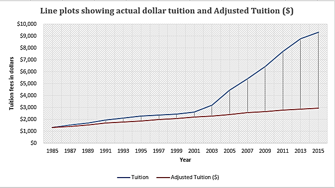
Interpretation: From the above two line plots on the same axes, it can be concluded that the constant dollar tuition has risen steadily from the year 1985 to the year 2015 but the actual dollar tuition for these years has increases sharply. So, it can be observed from the graph that the actual dollar tuition is increasing faster than the constant tuition dollar during the period 1985 to 2015.
Want to see more full solutions like this?
Chapter 16 Solutions
Statistics: Concepts and Controversies


- please find the answers for the yellows boxes using the information and the picture belowarrow_forwardA marketing agency wants to determine whether different advertising platforms generate significantly different levels of customer engagement. The agency measures the average number of daily clicks on ads for three platforms: Social Media, Search Engines, and Email Campaigns. The agency collects data on daily clicks for each platform over a 10-day period and wants to test whether there is a statistically significant difference in the mean number of daily clicks among these platforms. Conduct ANOVA test. You can provide your answer by inserting a text box and the answer must include: also please provide a step by on getting the answers in excel Null hypothesis, Alternative hypothesis, Show answer (output table/summary table), and Conclusion based on the P value.arrow_forwardA company found that the daily sales revenue of its flagship product follows a normal distribution with a mean of $4500 and a standard deviation of $450. The company defines a "high-sales day" that is, any day with sales exceeding $4800. please provide a step by step on how to get the answers Q: What percentage of days can the company expect to have "high-sales days" or sales greater than $4800? Q: What is the sales revenue threshold for the bottom 10% of days? (please note that 10% refers to the probability/area under bell curve towards the lower tail of bell curve) Provide answers in the yellow cellsarrow_forward
- Business Discussarrow_forwardThe following data represent total ventilation measured in liters of air per minute per square meter of body area for two independent (and randomly chosen) samples. Analyze these data using the appropriate non-parametric hypothesis testarrow_forwardeach column represents before & after measurements on the same individual. Analyze with the appropriate non-parametric hypothesis test for a paired design.arrow_forward
 MATLAB: An Introduction with ApplicationsStatisticsISBN:9781119256830Author:Amos GilatPublisher:John Wiley & Sons Inc
 Probability and Statistics for Engineering and th...StatisticsISBN:9781305251809Author:Jay L. DevorePublisher:Cengage Learning
 Statistics for The Behavioral Sciences (MindTap C...StatisticsISBN:9781305504912Author:Frederick J Gravetter, Larry B. WallnauPublisher:Cengage Learning
 Elementary Statistics: Picturing the World (7th E...StatisticsISBN:9780134683416Author:Ron Larson, Betsy FarberPublisher:PEARSON
 The Basic Practice of StatisticsStatisticsISBN:9781319042578Author:David S. Moore, William I. Notz, Michael A. FlignerPublisher:W. H. Freeman
 Introduction to the Practice of StatisticsStatisticsISBN:9781319013387Author:David S. Moore, George P. McCabe, Bruce A. CraigPublisher:W. H. Freeman