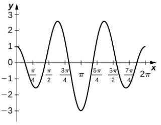
The following graph is of a function of the form f ( x ) = a cos ( n t ) + b cos ( m t ) . Estimate the coefficients a and b and the frequency parameters n and m. Use these estimates to approximate ∫ 0 π f ( t ) d t .
The following graph is of a function of the form f ( x ) = a cos ( n t ) + b cos ( m t ) . Estimate the coefficients a and b and the frequency parameters n and m. Use these estimates to approximate ∫ 0 π f ( t ) d t .
The following graph is of a function of the form
f
(
x
)
=
a
cos
(
n
t
)
+
b
cos
(
m
t
)
. Estimate the coefficients a and b and the frequency parameters n and m. Use these estimates to approximate
∫
0
π
f
(
t
)
d
t
.
Starting with the finished version of Example 6.2, attached, change the decision criterion to "maximize expected utility," using an exponential utility function with risk tolerance $5,000,000. Display certainty equivalents on the tree.
a. Keep doubling the risk tolerance until the company's best strategy is the same as with the EMV criterion—continue with development and then market if successful.
The risk tolerance must reach $ ____________ before the risk averse company acts the same as the EMV-maximizing company.
b. With a risk tolerance of $320,000,000, the company views the optimal strategy as equivalent to receiving a sure $____________ , even though the EMV from the original strategy (with no risk tolerance) is $ ___________ .
A Problem Solving Approach To Mathematics For Elementary School Teachers (13th Edition)
Knowledge Booster
Learn more about
Need a deep-dive on the concept behind this application? Look no further. Learn more about this topic, subject and related others by exploring similar questions and additional content below.
Area Between The Curve Problem No 1 - Applications Of Definite Integration - Diploma Maths II; Author: Ekeeda;https://www.youtube.com/watch?v=q3ZU0GnGaxA;License: Standard YouTube License, CC-BY


 College Algebra (MindTap Course List)AlgebraISBN:9781305652231Author:R. David Gustafson, Jeff HughesPublisher:Cengage Learning
 Trigonometry (MindTap Course List)TrigonometryISBN:9781337278461Author:Ron LarsonPublisher:Cengage Learning
 Trigonometry (MindTap Course List)TrigonometryISBN:9781305652224Author:Charles P. McKeague, Mark D. TurnerPublisher:Cengage Learning
 Algebra & Trigonometry with Analytic GeometryAlgebraISBN:9781133382119Author:SwokowskiPublisher:Cengage