Videos
State the null and alternative hypothesis.
Find the degrees of freedom for the
Find the critical value of chi-square from Appendix E or from Excel’s
Calculate the chi-square test statistics at 0.05 level of significance.
Interpret the p-value.
Check whether the conclusion is sensitive to the level of significance chosen, identify the cells that contribute to the chi-square test statistic and check for the small expected frequencies.
Perform a two-tailed, two-sample z test for
Answer to Problem 30CE
The null hypothesis is:
And the alternative hypothesis is:
The degrees of freedom for the contingency table is 1.
The critical-value using EXCEL is 3.841.
The chi-square test statistics at 0.05 level of significance is 1.50.
The p-value for the hypothesis test is 0.221.
There is enough evidence to conclude that the correct response and type of cola are independent.
The conclusion is not sensitive to the level of significance chosen.
The cells (1, 1) and (1, 2) contribute the most to the chi-square test statistic.
There is no expected frequencies that are too small.
It is verified that
Explanation of Solution
The table summarizes the grade and order of papers handed in.
The claim is to test whether the data provide sufficient evidence to conclude that the grade and order handed in are independent. If the claim is rejected, then the grade and order handed in are not independent.
The test hypotheses are given below:
Null hypothesis:
Alternative hypothesis:
The degrees of freedom can be obtained as follows:
Substitute 2 for r and 2 for c.
Thus, the degrees of freedom for the contingency table is 1.
Procedure for critical-value using EXCEL:
Step-by-step software procedure to obtain critical-value using EXCEL software is as follows:
- Open an EXCEL file.
- In cell A1, enter the formula “=CHISQ.INV.RT(0.05,1)”
- Output using EXCEL software is given below:
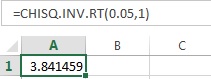
Thus, the critical-value using EXCEL is 3.841.
Test statistic:
Software procedure:
Step by step procedure to obtain the chi-square test statistics and p-value using the MINITAB software:
- Choose Stat > Tables >Cross Tabulation and Chi-Square.
- Choose Row data (categorical variables).
- In Rows, choose Grade.
- In Columns, choose Order handed in.
- In Frequencies, choose Count.
- In Display, select Counts.
- In chi-square, select Chi-square test, Expected cell counts and Each cell’s contribution to chi-square.
- Click OK.
Output using the MINITAB software is given below:
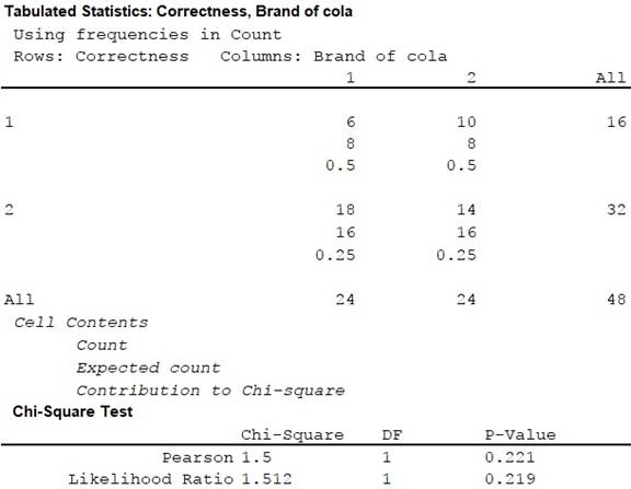
Thus, the test statistic is 1.50 and the p-value for the hypothesis test is 0.221.
Rejection rule:
If the p-value is less than or equal to the significance level, then reject the null hypothesis
Conclusion:
Here, the p-value is greater than the level of significance.
That is,
Therefore, the null hypothesis is not rejected.
Thus, the data provide sufficient evidence to conclude that the correct response and type of cola are independent.
Take
Here, the p-value is greater than the level of significance.
That is,
Therefore, the null hypothesis is not rejected.
Thus, the data provide sufficient evidence to conclude that the correct response and type of cola are independent.
Thus, the conclusion is same for both the significance levels.
Hence, the conclusion is not sensitive to the level of significance chosen.
The cells (1, 1) and (1, 2) contribute the most to the chi-square test statistic.
Since all
Two-tailed, two-sample z test:
The test hypotheses are given below:
Null hypothesis:
Alternative hypothesis:
The proportion of “yes” responses to the regular cola is denoted as
Where
The proportion of number of “yes” responses to the diet cola is denoted as
Where
The pooled proportion is denoted as
Test statistic:
The z-test statistics can be obtained as follows:
Thus, the z-test statistic is –1.22.
The square of the z-test statistic is,
Thus the square of the z-test statistic is same as the chi-square statistics.
Procedure for p-value using EXCEL:
Step-by-step software procedure to obtain p-value using EXCEL software is as follows:
- Open an EXCEL file.
- In cell A1, enter the formula “=2*(1-NORM.S.DIST(–1.22,1))”
- Output using EXCEL software is given below:
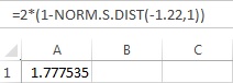
Thus, the p-value using EXCEL is 1.778, which is not same as the p-value obtained in chi-square test. But the square of the z-test statistic is same as the chi-square statistics.
Thus, it is verified that
Want to see more full solutions like this?
Chapter 15 Solutions
Gen Combo Ll Applied Statistics In Business & Economics; Connect Access Card


- Please help me with the following question on statisticsFor question (e), the drop down options are: (From this data/The census/From this population of data), one can infer that the mean/average octane rating is (less than/equal to/greater than) __. (use one decimal in your answer).arrow_forwardHelp me on the following question on statisticsarrow_forward3. [15] The joint PDF of RVS X and Y is given by fx.x(x,y) = { x) = { c(x + { c(x+y³), 0, 0≤x≤ 1,0≤ y ≤1 otherwise where c is a constant. (a) Find the value of c. (b) Find P(0 ≤ X ≤,arrow_forwardNeed help pleasearrow_forward7. [10] Suppose that Xi, i = 1,..., 5, are independent normal random variables, where X1, X2 and X3 have the same distribution N(1, 2) and X4 and X5 have the same distribution N(-1, 1). Let (a) Find V(X5 - X3). 1 = √(x1 + x2) — — (Xx3 + x4 + X5). (b) Find the distribution of Y. (c) Find Cov(X2 - X1, Y). -arrow_forward1. [10] Suppose that X ~N(-2, 4). Let Y = 3X-1. (a) Find the distribution of Y. Show your work. (b) Find P(-8< Y < 15) by using the CDF, (2), of the standard normal distribu- tion. (c) Find the 0.05th right-tail percentage point (i.e., the 0.95th quantile) of the distri- bution of Y.arrow_forward6. [10] Let X, Y and Z be random variables. Suppose that E(X) = E(Y) = 1, E(Z) = 2, V(X) = 1, V(Y) = V(Z) = 4, Cov(X,Y) = -1, Cov(X, Z) = 0.5, and Cov(Y, Z) = -2. 2 (a) Find V(XY+2Z). (b) Find Cov(-x+2Y+Z, -Y-2Z).arrow_forward1. [10] Suppose that X ~N(-2, 4). Let Y = 3X-1. (a) Find the distribution of Y. Show your work. (b) Find P(-8< Y < 15) by using the CDF, (2), of the standard normal distribu- tion. (c) Find the 0.05th right-tail percentage point (i.e., the 0.95th quantile) of the distri- bution of Y.arrow_forward== 4. [10] Let X be a RV. Suppose that E[X(X-1)] = 3 and E(X) = 2. (a) Find E[(4-2X)²]. (b) Find V(-3x+1).arrow_forward2. [15] Let X and Y be two discrete RVs whose joint PMF is given by the following table: y Px,y(x, y) -1 1 3 0 0.1 0.04 0.02 I 2 0.08 0.2 0.06 4 0.06 0.14 0.30 (a) Find P(X ≥ 2, Y < 1). (b) Find P(X ≤Y - 1). (c) Find the marginal PMFs of X and Y. (d) Are X and Y independent? Explain (e) Find E(XY) and Cov(X, Y).arrow_forward32. Consider a normally distributed population with mean μ = 80 and standard deviation σ = 14. a. Construct the centerline and the upper and lower control limits for the chart if samples of size 5 are used. b. Repeat the analysis with samples of size 10. 2080 101 c. Discuss the effect of the sample size on the control limits.arrow_forwardConsider the following hypothesis test. The following results are for two independent samples taken from the two populations. Sample 1 Sample 2 n 1 = 80 n 2 = 70 x 1 = 104 x 2 = 106 σ 1 = 8.4 σ 2 = 7.6 What is the value of the test statistic? If required enter negative values as negative numbers (to 2 decimals). What is the p-value (to 4 decimals)? Use z-table. With = .05, what is your hypothesis testing conclusion?arrow_forwardarrow_back_iosSEE MORE QUESTIONSarrow_forward_ios
 Big Ideas Math A Bridge To Success Algebra 1: Stu...AlgebraISBN:9781680331141Author:HOUGHTON MIFFLIN HARCOURTPublisher:Houghton Mifflin Harcourt
 Glencoe Algebra 1, Student Edition, 9780079039897...AlgebraISBN:9780079039897Author:CarterPublisher:McGraw Hill
 Holt Mcdougal Larson Pre-algebra: Student Edition...AlgebraISBN:9780547587776Author:HOLT MCDOUGALPublisher:HOLT MCDOUGAL